%%% Usage: Lucas_Kanade(
'1.bmp'
,
'2.bmp'
,10)
%%%%%%%%%%%%%%%%%%%%%%%%%%%%%%%%%%%%%%%%%%%%%%%%%%%%%%%%
%%%file1:输入图像1
%%%file2:输入图像2
%%%density:显示密度
function Lucas_Kanade(file1, file2, density)
%%% Read Images %% 读取图像
img1 = im2double (imread (file1));
%%% Take alternating rows and columns %% 按行分成奇偶
[odd1, ~] = split (img1);
img2 = im2double (imread (file2));
[odd2, ~] = split (img2);
%%% Run Lucas Kanade %% 运行光流估计
[Dx, Dy] = Estimate (odd1, odd2);
%%% Plot %% 绘图
figure;
[maxI,maxJ] = size(Dx);
Dx = Dx(1:density:maxI,1:density:maxJ);
Dy = Dy(1:density:maxI,1:density:maxJ);
quiver(1:density:maxJ, (maxI):(-density):1, Dx, -Dy, 1);
axis square;
%%% Run Lucas Kanade on all levels and interpolate %% 光流
function [Dx, Dy] = Estimate (img1, img2)
level = 4;%%%金字塔层数
half_window_size = 2;
% [m, n] = size (img1);
G00 = img1;
G10 = img2;
if
(level > 0)%%%从零到level
G01 = reduce (G00); G11 = reduce (G10);
end
if
(level>1)
G02 = reduce (G01); G12 = reduce (G11);
end
if
(level>2)
G03 = reduce (G02); G13 = reduce (G12);
end
if
(level>3)
G04 = reduce (G03); G14 = reduce (G13);
end
l = level;
for
i = level: -1 :0,
if
(l == level)
switch
(l)
case
4, Dx = zeros (size (G04)); Dy = zeros (size (G04));
case
3, Dx = zeros (size (G03)); Dy = zeros (size (G03));
case
2, Dx = zeros (size (G02)); Dy = zeros (size (G02));
case
1, Dx = zeros (size (G01)); Dy = zeros (size (G01));
case
0, Dx = zeros (size (G00)); Dy = zeros (size (G00));
end
else
Dx = expand (Dx);
Dy = expand (Dy);
Dx = Dx .* 2;
Dy = Dy .* 2;
end
switch
(l)
case
4,
W = warp (G04, Dx, Dy);
[Vx, Vy] = EstimateMotion (W, G14, half_window_size);
case
3,
W = warp (G03, Dx, Dy);
[Vx, Vy] = EstimateMotion (W, G13, half_window_size);
case
2,
W = warp (G02, Dx, Dy);
[Vx, Vy] = EstimateMotion (W, G12, half_window_size);
case
1,
W = warp (G01, Dx, Dy);
[Vx, Vy] = EstimateMotion (W, G11, half_window_size);
case
0,
W = warp (G00, Dx, Dy);
[Vx, Vy] = EstimateMotion (W, G10, half_window_size);
end
[m, n] = size (W);
Dx(1:m, 1:n) = Dx(1:m,1:n) + Vx; Dy(1:m, 1:n) = Dy(1:m, 1:n) + Vy;
smooth (Dx);
smooth (Dy);
l = l - 1;
end
%%% Lucas Kanade on the image sequence at pyramid step %%
function [Vx, Vy] = EstimateMotion (W, G1, half_window_size)
[m, n] = size (W);
Vx = zeros (size (W)); Vy = zeros (size (W));
N = zeros (2*half_window_size+1, 5);
for
i = 1:m,
l = 0;
for
j = 1-half_window_size:1+half_window_size,
l = l + 1;
N (l,:) = getSlice (W, G1, i, j, half_window_size);
end
replace = 1;
for
j = 1:n,
t = sum (N);
[v, d] = eig ([t(1) t(2);t(2) t(3)]);
namda1 = d(1,1); namda2 = d(2,2);
if
(namda1 > namda2)
tmp = namda1; namda1 = namda2; namda2 = tmp;
tmp1 = v (:,1); v(:,1) = v(:,2); v(:,2) = tmp1;
end
if
(namda2 < 0.001)
Vx (i, j) = 0; Vy (i, j) = 0;
elseif (namda2 > 100 * namda1)
n2 = v(1,2) * t(4) + v(2,2) * t(5);
Vx (i,j) = n2 * v(1,2) / namda2;
Vy (i,j) = n2 * v(2,2) / namda2;
else
n1 = v(1,1) * t(4) + v(2,1) * t(5);
n2 = v(1,2) * t(4) + v(2,2) * t(5);
Vx (i,j) = n1 * v(1,1) / namda1 + n2 * v(1,2) / namda2;
Vy (i,j) = n1 * v(2,1) / namda1 + n2 * v(2,2) / namda2;
end
N (replace, :) = getSlice (W, G1, i, j+half_window_size+1, half_window_size);
replace = replace + 1;
if
(replace == 2 * half_window_size + 2)
replace = 1;
end
end
end
%%% The Reduce Function
for
pyramid %%金字塔压缩
function result = reduce (ori)
[m,n] = size (ori);
mid = zeros (m, n);
%%%行列值的一半
m1 = round (m/2);
n1 = round (n/2);
%%%输出即为输入图像的1/4
result = zeros (m1, n1);
%%%滤波
%%%0.05 0.25 0.40 0.25 0.05
w = generateFilter (0.4);
for
j = 1 : m,
tmp = conv([ori(j,n-1:n) ori(j,1:n) ori(j,1:2)], w);
mid(j,1:n1) = tmp(5:2:n+4);
end
for
i=1:n1,
tmp = conv([mid(m-1:m,i); mid(1:m,i); mid(1:2,i)]', w);
result(1:m1,i) = tmp(5:2:m+4)';
end
%%% The Expansion Function
for
pyramid %%金字塔扩展
function result = expand (ori)
[m,n] = size (ori);
mid = zeros (m, n);
%%%行列值的两倍
m1 = m * 2;
n1 = n * 2;
%%%输出即为输入图像的4倍
result = zeros (m1, n1);
%%%滤波
%%%0.05 0.25 0.40 0.25 0.05
w = generateFilter (0.4);
for
j=1:m,
t = zeros (1, n1);
t(1:2:n1-1) = ori (j,1:n);
tmp = conv ([ori(j,n) 0 t ori(j,1) 0], w);
mid(j,1:n1) = 2 .* tmp (5:n1+4);
end
for
i=1:n1,
t = zeros (1, m1);
t(1:2:m1-1) = mid (1:m,i)';
tmp = conv([mid(m,i) 0 t mid(1,i) 0], w);
result(1:m1,i) = 2 .* tmp (5:m1+4)';
end
function filter = generateFilter (alpha)%%%滤波系数
filter = [0.25-alpha/2, 0.25, alpha, 0.25, 0.25-alpha/2];
function [N] = getSlice (W, G1, i, j, half_window_size)
N = zeros (1, 5);
[m, n] = size (W);
for
y = -half_window_size:half_window_size,
Y1 = y +i;
if
(Y1 < 1)
Y1 = Y1 + m;
elseif (Y1 > m)
Y1 = Y1 - m;
end
X1 = j;
if
(X1 < 1)
X1 = X1 + n;
elseif (X1 > n)
X1 = X1 - n;
end
DeriX = Derivative (G1, X1, Y1,
'x'
); %%%计算x、y方向梯度
DeriY = Derivative (G1, X1, Y1,
'y'
);
N = N + [ DeriX * DeriX, ...
DeriX * DeriY, ...
DeriY * DeriY, ...
DeriX * (G1 (Y1, X1) - W (Y1, X1)), ...
DeriY * (G1 (Y1, X1) - W (Y1, X1))];
end
function result = smooth (img)
result = expand (reduce (img));%%%太碉
function [odd, even] = split (img)
[m, ~] = size (img);%%%按行分成奇偶
odd = img (1:2:m, :);
even = img (2:2:m, :);
%%% Interpolation %% 插值
function result = warp (img, Dx, Dy)
[m, n] = size (img);
[x,y] = meshgrid (1:n, 1:m);
x = x + Dx (1:m, 1:n);
y = y + Dy (1:m,1:n);
for
i=1:m,
for
j=1:n,
if
x(i,j)>n
x(i,j) = n;
end
if
x(i,j)<1
x(i,j) = 1;
end
if
y(i,j)>m
y(i,j) = m;
end
if
y(i,j)<1
y(i,j) = 1;
end
end
end
result = interp2 (img, x, y,
'linear'
);%%%二维数据内插值
%%% Calculates the Fx Fy %% 计算x、y方向梯度
function result = Derivative (img, x, y, direction)
[m, n] = size (img);
switch
(direction)
case
'x'
,
if
(x == 1)
result = img (y, x+1) - img (y, x);
elseif (x == n)
result = img (y, x) - img (y, x-1);
else
result = 0.5 * (img (y, x+1) - img (y, x-1));
end
case
'y'
,
if
(y == 1)
result = img (y+1, x) - img (y, x);
elseif (y == m)
result = img (y, x) - img (y-1, x);
else
result = 0.5 * (img (y+1, x) - img (y-1, x));
end
end


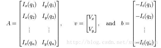
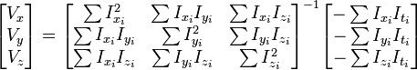
 ,
,  和
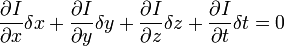
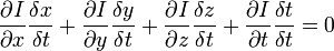
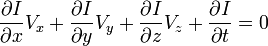
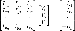
和  则是图像在(x ,y ,z ,t )这一点向相应方向的差分 。
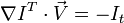


 or
or
 来突出窗口中心点的坐标。


