注:此文为复现sim-GAN,参考了一些论文,博客,如有侵权请联系,我附上原出处。
由于一些格式原因,文章有些部分会比较乱,请见谅。
Learning from Simulated and Unsupervised Images through Adversarial Training
通过对抗的训练来从模拟和无监督图像中学习
摘要
[摘要] 随着计算机视觉的进步,在合成图像上训练模型变得更容易处理,可能避免需要昂贵的注释。然而,由于合成图像和真实图像分布之间的差距,从合成图像学习可能无法实现预期的性能。为了减少这种差距,本文实现了最近十分流行(模拟+无监督)学习Simulated+Unsupervised(S+U)learning,其任务是学习模型以使用未标记的真实数据改善模拟器输出的真实性,同时保留模拟器中的注释信息。使用了一种S + U学习方法,该方法使用类似于生成对抗网络(GAN)的对抗网络,但使用合成图像作为输入而不是随机向量。(模拟+无监督)学习对传统的GAN算法进行了几项关键修改,以保留注释,避免人造痕迹并保持稳定性:(i)自我正规化,(ii)局部对抗性损失,(iii)利用历史缓冲区的细化图片来更新判别器。实验结果表明,这可以生成高度逼真的图像。
[关键词] 生成对抗网络; (模拟+无监督)学习; 深度学习
第1章 引言
1.1背景介绍与研究意义
随着近来深度神经网络的兴起,大型的标记训练数据集变得越来越重要。然而,标记这样大的数据集是昂贵且耗时的。因此,对合成而非真实图像进行训练的想法变得有吸引力,因为其是自动可用的。
然而,由于合成图像和实际图像分布之间的差距,从合成图像中学习可能是有问题的。合成数据通常不够真实,导致网络学习仅存在于合成图像中的细节并且不能在真实图像上很好地概括。缩小这一差距的一个解决方案是改进模拟器。然而,增加真实感通常在计算上是昂贵的,渲染器设计需要大量的努力,甚至顶级渲染器仍然可能无法模拟真实图像的所有特征。这种现实细节的缺乏可能会导致模型在合成图像中超出“不现实”的细节。

如图1,在本文中,采用了模拟+无监督(S + U)学习,其目标是使用未标记的实际数据来改善细化器中合成图像的真实性。改进的真实性使得能够在大型数据集上训练更好的机器学习模型,而无需任何数据收集或人工标记工作。除了增加真实感外,S + U学习还应保留用于训练机器学习模型的标注信息,例如应该保留图1中的凝视方向。此外,由于机器学习模型可能对合成数据中的人造痕迹敏感,因此S + U学习应该生成没有人造痕迹的图像。
S+U学习方法(SimGAN):用一个细化器(细化网络refiner network)来细化合成图像,概述见图2,合成图像由黑箱模拟器生成,并经细化网络细化。
(i)为增加真实度,类似GANs训练对抗网络,用正则损失,使判别网络无法区分细化的生成图像与真实图像。
(ii)为保留合成图像的标注,为对抗损失补充自正则损失,来惩罚合成图像与真实图像间的巨大改变。进一步用一全卷积网络操作像素并保留全局结构(而非如全连接编码网络那样去完全改变图像内容)。
(iii)GAN框架用竞争的目标来训练2个网络,使网络不稳定且易引入合成现象。因此限制判别器的感受野至局部区域(而非整幅图像),使每幅图有多个局部的对抗损失。并用细化图像的历史(而非当前细化网络输出的细化图像)更新判别器来稳定训练。

1.2研究内容与目标
本实验研究内容主要是基于SimGAN网络的人眼数据生成方法及系统,提升人眼数据的真实度。
本实验目标主要有两个:一方面是,在可用数据集上基于SimGAN网络训练出一个较好的人眼数据生成模型;另一方面是, 在python 上开发构建出一个人眼数据训练与生成系统,实现:一、对图片的人眼进行识别分割,输出仅含人眼数据的可用数据集,二、对合成的人眼数据进行提升真实度操作。
第2章 GAN网络原理
2.1 GAN网络
对抗生成网络GAN(Generative Adversarial Networks)。原始的GAN是一种无监督学习方法,它巧妙地利用“对抗”的思想来学习生成式模型,一旦训练完成后可以生成全新的数据样本,是近年来复杂分布上无监督学习最具前景的方法之一。
GAN的基本原理非常简单。生成器G的输入是一个n维向量,包含有各种待生成的图片的标签信息等,将该向量添加一个噪声后送入生成器中,生成器生成图片送入判别器D中,由判别器判断这张图片是真实的还是虚假的,(通常情况下,若输出为1,判断图片为真实,而输出为0,判断图片为虚假)。
若将生成器生成的图片判断为虚假的,则生成器需要优化参数来生成更加逼真的,能够欺骗判别器的图片;若被判断为是真实的,则判别器需要优化参数来更准确的判断送入的图像。生成器生成的样本和真实样本是交替的送入判别器中的。
这样生成器G和判别器D构成了一个动态的“博弈”,这是GAN的基本思想。

最后博弈的结果是什么?在最理想的状态下,生成器G可以生成足以“以假乱真”的图片G(z)。 对于判别器D来说,它难以判定生成器G生成的图片究竟是不是真实的,因此D(G(z))=0.5。此时得到了一个生成式的模型,它可以用来生成图片。
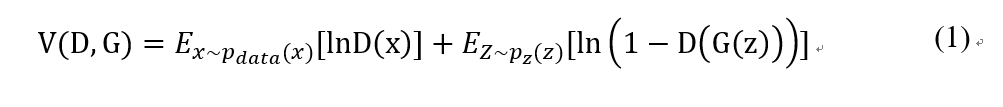
下面用数学化的语言来描述这个过程。假设用于训练的真实图片数据是x,图片数据的分布为p_data (x),之前说生成器G能够“生成图片”,实际是生成器G可以学习到的真实数据分布p_data (x)。 噪声z的分布设为p_z (x),p_z (x)是已知的,而p_data (x)是未知的。在理想情况下,G(z)的分布应该尽可能接近p_data (x),生成器G将已知分布的z变量映射到了未知分布x变量上。
注:关于交叉熵的理解,可以参考
https://blog.csdn.net/tsyccnh/article/details/79163834
写得挺好的
根据交叉摘损失,可以构造下面的损失函数


2.1 卷积神经网络
卷积神经网络(Convolutional Neural Networks, CNN)是一类包含卷积计算且具有深度结构的前馈神经网络,是深度学习的代表算法之一。卷积神经网络具有特征学习能力,能够按其阶层结构对输入信息进行平移不变分类,因此也被称为“平移不变人工神经网络”。
2.1.1 卷积层
卷积神经网络用卷积层提取特征。卷积层由一个卷积核(kernel),参数步长(stride)和补齐操作(pad)。卷积运算就是卷积核在二维图像上滑动,将卷积核覆盖图像区域像素于对应卷积核的值相乘后再一起相加作为输出。如图2-1所示。

2.1.2 池化层
池化层(pooling layer)是卷积神经网络一个重要操作,也称为下采样。主要用于特征降维,压缩数据和参数的数量,减小过拟合,同时提高模型的容错性。和卷积层类似,有kernel_size、stride和pad两个参数。最常见的池化层有最大池化和平均池化。平均池化是取这个范围内平均值,而最大池化就取kernel_size × kernel_size范围内的最大值。如图2-2所示。

2.1.3 激活函数层
激活函数主要来做非线性变换,前面卷积层、pooling层都是线性的,如果没有激活函数,整个网络都是线性的,训练模型效果较差。加入激活函数,可以加快训练速度,使模型更具鲁棒性。常见激活函数主要有Sigmoid、Relu等。Sigmoid激活函数在两端梯度几乎为0,如果输入数据过大或过小,会导致梯度消散现象发生。Relu激活函数就是为了解决这个问题,在大于0的时候导数为1,小于0时候为0,因为训练时候小于零情况较少,所以能有效解决梯度消散的问题。
在训练网络时候,正常情况下把激活函数放在卷积层后面,不同激活函数用于不同任务。

2.2残差网络((Residual Networks, ResNets)
残差网络是由来自Microsoft Research的4位学者提出的卷积神经网络。残差网络的特点是容易优化,并且能够通过增加相当的深度来提高准确率。其内部的残差块使用了跳跃连接,缓解了在深度神经网络中增加深度带来的梯度消失问题。
可以看到x=Input Features是这一残差块的输入,也称作F(x)为残差,x为输入值,F(X)是经过第一层线性变化并激活后的输出,该图表示在残差网络中,第二层进行线性变化之后激活之前,F(x)加入了这一层输入值X,然后再进行激活后输出。在第二层输出值激活前加入X,这条路径称作shortcut连接。

shortcut layer是F(x)+x的实现层,F(x)输出尺寸如果和原来输入 x 维度一样,则直接相加,否则尺度较小的需要用0填充或使用1×1卷积进行变换。
残差网络结构设计巧妙,通过两层或多次的跳越进行短接,有效解决了深度网络退化问题。
2.3小结
卷积神经网络与全连接层网络相比的优点:1、参数共享2、稀疏连接。它只与图像中的一个区域有关,与其他区域(像素点)无关,因此减小了参数。并且,卷积神经网络善于捕捉平移不变性(移动后的结构特征依然明显),因此是否适合用于提取图像特征。
最大池化,选取根由特征的点保留下来,以此达到尽可能提取更多特征的效果。
通常情况下,非常深的网络难以训练,因为存在梯度消失和梯度爆炸。残差网络通过跳远连接,有效传递了参数,能够更好的训练网络。
第3章 SimGAN原理
3.1. 使用SimGAN的S+U学习

3.2 细化网络结构
细化网络(细化器refiner network)为残差网络:包括3×3大小的滤波器卷积55×35大小的输入图像,输出64个特征图。输出经过4个残差模块。最后1个残差模块的输出经过1个1×1大小的卷积层来输出1个对应细化的合成图像的特征图,如图。

每个残差网络模块包含2个卷积层,每个卷积层包含64个特征图,如图。

细化网络的作用:合成图像送入细化器中,细化器通过学习到的真实图像的特征,对合成图像进行修正,它在像素级别修改合成图像,而不是整体修改图像内容,保留全局结构和注释,添加一些逼真的细节。
3.3 判别网络结构

3.4损失函数


3.4.1自正则的对抗损失
除生成逼真图像,细化网络应保留模拟器的标注信息(生成器的特征信息)。如,生成人眼图像时:学到的变换不应改变注视方向。因而使机器学习模型能用有标注信息(特征信息)的细化图像。为此,提出自正则(Self-Regularization)损失来最小化合成图像与细化图像间的图像差异。
因此,方程(3)中的全部损失函数公式为:

3.4.2 局部的对抗损失
训练单个判别网络时,细化网络往往过分强调特定的图像特征来欺骗当前的判别网络。从细化图像中采样的局部块应与真实图像中的对应块有相似的统计特性。因此,定义可单独分类所有图像块的判别网络(而非全局判别网络)。这样限制了感受区域的大小(判别网络的容量);为学习判别网络提供更多的样本;更好地训练细化网络(因为每幅图像都有多个“真实度损失”)。

如图3-2,在实现中,设计判别网络D输出w×h概率图,判断输入块是否为合成图像。其中,w×h为图像中局部块的数目。训练细化网络时,对抗性损失是w×h个局部块上求和交叉熵损失的总和。
3.5. 用细化图像历史缓冲区来更新判别网络
对抗训练另一问题:判别网络仅关注最近时间步上的细化图像。这可能导致:(i)训练发散,(ii)细化网络引入判别网络无法发现的合成现象。
对于判别网络,整个训练中所有时间步上,所有细化网络生成的细化合成图像都为合成图像。因此,判别网络应能将所有这些图像分类为合成图像。基于此,用细化图像的历史缓冲来更新判别网络,以此提高训练的稳定性(而非仅用当前时间步上的小块)。

3.6 对抗训练算法

训练判别网络时每次迭代,从当前细化网络和图像缓冲中分别采样b/2张图像来更新参数ϕ。固定缓冲大小B。每次迭代后,每次迭代之后,随机的将缓冲中的b/2的样本替换成新生成的细化图像。
3.4 小结
通过对SimGAN算法流程的研究理解,可以看出(S+U)学习在数据生成方面有重要作用。
首先,实验使用局部对抗性损失训练。因为全局对抗性损失在判别网络中使用完全连接的层,将整个图像分类为真实的和合成的。其次,相比于传统的GAN网络的损失函数,SimGAN在损失函处多加了一个正则化项,这个正则化项的目的是惩罚细化合成图像和原始合成图像之间的巨大差别,避免细化网络在细化合成图片的时候用力过猛修改了原图像的内容。局部对抗性损失消除了伪影并使生成的图像显着更逼真。接下来,如图3-5,利用图像缓冲历史来优化网络,使用缓冲器完成的图像可以在标准训练中防止严重的伪影。比如,在眼角的部分[1]。
第4章 实验结果分析
4.1 实验设置
本实验部分的环境配置如表4-1所示。

合成人眼训练数据集为UnityEyes数据集,真实人眼训练数据集MPIIGaze数据集,batch size为49,在英伟达NVIDIA GeForce 940MX显卡上训练模型,梯度下降算法采用SGD,学习速率设置为0.001,迭代次数为8000次,训练时间为20小时。
4.2 数据集
本课题采用的数据集UnityEyes[3]、MPIIGaze[4]。UnityEyes用来模拟人眼图片,MPIIGaze用来训练模型,学习人眼特征。
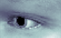
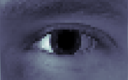
UnityEyes 数据集是剑桥大学计算机实验室提供的数据集。它使用生成3D眼睛区域模型渲染了一百万个眼睛图像。这些合成图像(右下)使用简单的k-最近邻方法进行凝视估计,与实际输入图像(右上)匹配,如图4-9。

MPIIGaze数据集,其中包含213,659个全脸图像以及在日常笔记本电脑使用期间从几个月内收集的15个用户的相应地面真实注视位置。体验采样方法确保了连续的凝视和头部姿势以及眼睛外观和照明的真实变化。

4.3 评估指标
训练细化网络和判别网络的误差收敛。
4.4 实验结果分析
参数解释:
(img_width = 55,img_height = 35,img_channels = 1)(55351)
nb_steps(迭代次数)
batch_size(批量图片数)
log_interval(更新间隔)
pre_steps(预训练次数)
k_d(每步的判别网络更新次数)
k_g(每步的细化网络更新次数)
实验一、
参数设置:batch_size=49,log_interval=100,pre_steps=15,k_d=1,k_g=2
在修改nb_steps的情况下进行实验
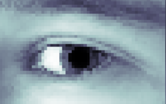
表4-2 不同迭代次数下的细化合成情况
| nb_steps |
细化合成图像节选 |
Refiner model loss |
Discriminator model loss refined |
| 100 |
 |
[1.78107663 1.08891018 0.69216645] |
[0.34716649] |
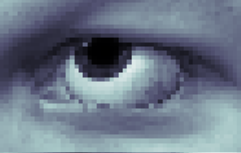
| 500 |
 |
[0.90662724 0.22514614 0.6814811 ] |
[0.3526878] |
| 1000 |
 |
[0.84306497 0.17703002 0.66603495] |
[0.3611398] |
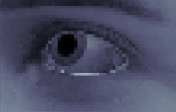
| 2000 |
 |
[0.76847622 0.13664375 0.63183247] |
[0.38209656] |
| 3000 |
 |
[0.72315078 0.11662279 0.606528 ] |
[0.40196903] |
| 4000 |
 |
[0.70487172 0.10420461 0.60066711] |
[0.40952167] |
| 5000 |
 |
[0.69427984 0.09646344 0.5978164 ] |
[0.41345715] |
| 6000 |
 |
[0.68985704 0.09063611 0.59922092] |
[0.41556636] |
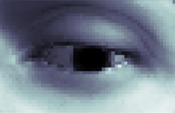
| 7000 |
 |
[0.68767308 0.08596543 0.60170765] |
[0.4166556] |
| 8000 |
 |
[0.6885478 0.08269296 0.60585485] |
[0.41424642] |
由表4-1可见,随着迭代次数的增加,损失越来越小,模型的真实度也由所提升。
可用看到,1000次时细化网络为合成图片添加了皮肤纹理,皱纹,学习到了2000次时添加了眼球高光。学习到了8000次时,误差以逐渐收敛。
实验二、
参数设置:nb_steps=100,log_interval=100,pre_steps=15,k_d=1,k_g=2
在修改batch_size的情况下进行实验

增加了batch_size的大小,损失函数并没有明显降低,但运行时间明显增长,考虑到网络采用的是局部损失而不是全局损失,也许一次批处理的量的大小并没有那么重要,但是并不绝对,要结合实际数据集进行分析,比如特征较少的数据可用适量添加batch_size的大小,防止过拟合的同时,运行时间差异也不会如此大。在人眼数据集下,
建议使用较小的batch_size。
实验三、
参数设置:nb_steps=100,batch_size=49,pre_steps=15,k_d=1,k_g=2
在修改log_interval的情况下进行实验

在log_interval减小的情况下,细化网络的损失有所下降,判别网络的损失基本不变,其实可用认为这是网络的震荡,因为log_interval虽然不同,但损失取得是每次间隔总和的平均值,因此,可用认为它们是大同小异的。
实验四、
参数设置:nb_steps=200,log_interval=100,batch_size=49,pre_steps=15,k_d=1,k_g=2
在修改数据集大小的情况下进行实验

在数据集较大的情况下,细化网络和判别网络的损失明显下降,这也侧面反应了(S+U)学习的缺点,(S+U)学习需要一个相当大的真实数据集来对合成图片进行优化。
实验五、
参数设置:nb_steps=100,log_interval=100,batch_size=49,k_d=1,k_g=2
在修改pre_steps的情况下进行实验

在增加pre_steps的情况下,细化网络和判别网络的损失基本不变,从侧面反映,(S+U)学习的主要优化实在后面的正式训练,在达到一定的迭代次数后,不同pre_steps的情况下的差异将会减小。
4.7 小结
根据上述实验结果,可以看出SimGAN算法相比于传统的GAN其他算法,SimGAN模型成功获取真实图像中皮肤纹理,传感器噪声和虹膜区域的外观。该方法提高真实度的同时,保留了标注信息(注视方向)。
首先,实验比较迭代次数,在迭代次数增加的情况下,生成的细化合成图片的真实度不断提升。但是也有需要克服的问题:1、生成的人眼图片较模糊 2、生成人眼图片的模型训练本身需要大量的数据集,能否使用较轻量的数据集。
由上述的人眼数据生成系统可以看出系统将数据生成和网络训练、界面融合为一体,可以实现基本的数据生成,模型训练,生成模拟真实人眼图像的功能。但是也还有需要完善的部分:1、如何在较短的时间训练出一个较好的模型。2、能否复现到其他数据集。
结 论
本文从的训练数据集需求出发,对基于SimGAN网络的人眼数据生成方法及系统,训练出可用生成真实度高的人眼数据,最后基于python的tkinter实现SimGAN网络下的人眼数据生成系统。
在SimGAN算法中,提出了模拟+无监督学习,以使用未标记的实际数据来细化模拟器的输出。S + U学习为模拟器增加了真实感,并保留了合成图像的全局结构和特征。但是由于学习是一个相对漫长的过程,所以对数据集的大小,机器的性能,时间的要求比较高。
在本次实验中,难以达到很好的生成训练图片的效果,在今后将会继续完善实验:1、如何在较短的时间训练出一个较好的模型。2、能否复现到其他数据集。
参考文献
[1] Ashish Shrivastava, Learning from Simulated and Unsupervised Images through Adversarial Training [J], CVPR, 2016.
[2] IanJ.Goodfellow, Generative Adversarial Nets. [J], CVPR, 2014.
[3] X. Zhang, Y. Sugano, M. Fritz, and A. Bulling. Appearance-based gaze estimation in the wild. In Proc. CVPR, 2015.
[4] E. Wood, T. Baltrušaitis, L. Morency, P. Robinson,andA.Bulling.Learninganappearance-based gaze estimator from one million synthesised images. In Proc. ACM Symposium on Eye Tracking Research & Applications, 2016.LeCun Y. LeNet-5, convolutional neural networks[EB/OL]. http://yann. lecun. com/exdb/lenet.2015, 20.
代码实现
代码出处:
https://github.com/mjdietzx/SimGAN
https://www.kaggle.com/kmader/simgan-notebook/data#Pretraining
注:数据集建议直接在第二个链接下下载,因为好像有一个数据集想直接下载的时候没有下载权限
建议使用GPU,基于python 3
代码我注释得很详细~
让我们再来理顺一下(我写的,有点丑,建议先自己看一遍代码,理解可能有错误):


import os
import sys
import keras
from keras import applications
from keras import layers
from keras import models
from keras import optimizers
from keras.preprocessing import image
import h5py
import numpy as np
import tensorflow as tf

print('tf-version', tf.__version__, 'keras-version', keras.__version__)
#
# directories
#

"""
加载数据
在这里我们设置路径并加载hdf5文件中的数据,因为否则会有太多单独的jpg / png图像
"""
path = os.path.dirname(os.path.abspath('.'))  # os.path.abspath(__file__)可以获得当前模块的绝对路径
# data_dir 数据集地址
data_dir = os.path.join('D:\workspace\Computer Vision\SimGAN-master', 'input')
# cache_dir 模型保存地址
cache_dir = 'D:\workspace\Computer Vision\SimGAN-master\cache'

# 加载数据文件并提取数据尺寸
with h5py.File(os.path.join(data_dir, 'gaze.h5'),'r') as t_file:
    print(list(t_file.keys()))
    assert 'image' in t_file, "Images are missing"
    assert 'look_vec' in t_file, "Look vector is missing"
    assert 'path' in t_file, "Paths are missing"
    print('Synthetic images found:',len(t_file['image']))
    for _, (ikey, ival) in zip(range(1), t_file['image'].items()):
        print('image',ikey,'shape:',ival.shape)
        img_height, img_width = ival.shape
        img_channels = 1
    # np.expand_dims 添加一行数据
    syn_image_stack = np.stack([np.expand_dims(a,-1) for a in t_file['image'].values()],0)

with h5py.File(os.path.join(data_dir, 'real_gaze.h5'),'r') as t_file:
    print(list(t_file.keys()))
    assert 'image' in t_file, "Images are missing"
    print('Real Images found:',len(t_file['image']))
    for _, (ikey, ival) in zip(range(1), t_file['image'].items()):
        print('image',ikey,'shape:',ival.shape)
        img_height, img_width = ival.shape
        img_channels = 1
    real_image_stack = np.stack([np.expand_dims(a,-1) for a in t_file['image'].values()],0)

#
#  训练参数
#

# nb_steps = 20
nb_steps = 1000    # originally 10000
batch_size = 100
k_d = 1  # number of discriminator updates per step 每步的 鉴别器 更新次数
k_g = 2  # number of generative network updates per step 每步的 细化器 更新次数
log_interval = 100  # 间隔
pre_steps = 15  # 用于预训练


"""
绘制图像以及相应的地面实况标签和模型预测标签,
绘制由GAN生成的图像以及用于生成这些图像的任何注释,
绘制合成,生成,精炼和真实的图像,看看它们如何在GAN中进行训练,
等等...
"""
import matplotlib
from matplotlib import pyplot as plt
from itertools import groupby
# from skimage.util.montage import montage2d
from skimage.util._montage import montage as montage2d


# plot_batch(
# image_batch    np.concatenate((synthetic_image_batch, refiner_model.predict_on_batch(synthetic_image_batch))),
# figure_path    os.path.join(cache_dir, figure_name),
# label_batch=None    label_batch=['Synthetic'] * batch_size + ['Refined'] * batch_size)
# 批量绘图 保存图片
def plot_batch(image_batch, figure_path, label_batch=None):
    all_groups = {label: montage2d(np.stack([img[:, :, 0] for img, lab in img_lab_list], 0))
                  for label, img_lab_list in groupby(zip(image_batch, label_batch), lambda x: x[1])}
    # 划分子图区域subplots
    fig, c_axs = plt.subplots(1, len(all_groups), figsize=(len(all_groups) * 4, 8), dpi=1600)
    # c_axs 子图
    for c_ax, (c_label, c_mtg) in zip(c_axs, all_groups.items()):
        c_ax.imshow(c_mtg, cmap='bone')
        # c_ax.imshow(c_mtg)
        c_ax.set_title(c_label)
        c_ax.axis('off')
    fig.savefig(os.path.join(figure_path))
    plt.close()


"""
实现论文2.3中描述的图像历史缓冲区的模块。
使用历史缓冲记录更新判别器
"""
# 图像历史缓冲区
class ImageHistoryBuffer(object):
    # 初始化
    def __init__(self, shape, max_size, batch_size):
        """
        初始化类的状态。
         :param shape:要存储在图像历史缓冲区中的数据的形状
                       (即(0,img_height,img_width,img_channels))。
         :param max_size:可以存储在历史缓冲区中的最大图片数。
         :param batch_size:用于训练GAN的批量大小。
        """
        self.image_history_buffer = np.zeros(shape=shape)
        self.max_size = max_size
        self.batch_size = batch_size

    def add_to_image_history_buffer(self, images, nb_to_add=None): # 添加图像到历史缓冲区
        """
        在GAN训练期间
        生成器生成一批新图像时,默认情况下,将batch_size // 2(batch_size 除二求整)个图像分别添加到图像历史记录缓冲
    :param images:要添加到图像历史缓冲区的图像数组(通常是批处理)。
    :param nb_to_add:要添加到图像历史缓冲区的`images`的图像数
                        (默认情况下为batch_size / 2)。
        """
        if not nb_to_add:
            nb_to_add = self.batch_size // 2
        if len(self.image_history_buffer) < self.max_size:
            np.append(self.image_history_buffer, images[:nb_to_add], axis=0)
        elif len(self.image_history_buffer) == self.max_size:
            self.image_history_buffer[:nb_to_add] = images[:nb_to_add]
        else:
            assert False
        np.random.shuffle(self.image_history_buffer)

    def get_from_image_history_buffer(self, nb_to_get=None):
        """
        从历史缓冲区中获取随机的图像样本。
     :param nb_to_get:从图片历史记录缓冲区获取的图片数(默认情况下为batch_size / 2)。
     :return:如果是图像,来自图像历史缓冲区的随机样本`nb_to_get`图像,
                    若为空np数组,则历史缓冲区为空。
        """
        if not nb_to_get:
            nb_to_get = self.batch_size // 2

        try:
            return self.image_history_buffer[:nb_to_get]
        except IndexError:
            return np.zeros(shape=0)

"""
网络架构
细化网络 refiner_network、判别网络 discriminator_network
他们互相攻击,不断提高对方的能力。
"""

# 细化网络
def refiner_network(input_image_tensor):
    """
    细化网络Rθ是残差网络(ResNet)。
    它改为在像素级别修改合成图像,而不是整体修改图像内容,保留全局结构和注释。
  :param input_image_tensor:与合成图像(synthetic image)对应的输入张量。
  :return:对应于精细合成图像(refined synthetic image)的输出张量。
    """

    def resnet_block(input_features, nb_features=64, nb_kernel_rows=3, nb_kernel_cols=3):
        """
        一个带有两个`nb_kernel_rows` x`nb_kernel_cols`卷积层的ResNet块,
         每个都有`nb_features`特征映射。
    请参阅论文中的图6。
    :param input_features:输入到ResNet块的张量。
    :return:来自ResNet块的输出张量。
        """
        # 卷积
        y = layers.Convolution2D(nb_features, nb_kernel_rows, nb_kernel_cols, border_mode='same')(input_features)
        y = layers.Activation('relu')(y)  # 激化函数relu
        y = layers.Convolution2D(nb_features, nb_kernel_rows, nb_kernel_cols, border_mode='same')(y)
        # 合并
        y = layers.merge([input_features, y], mode='sum')
        # y = layers.merge([input_features, y])
        return layers.Activation('relu')(y)

    # 大小为w×h的输入图像与输出64特征的3×3滤波器进行卷积 默认strides=(1, 1)
    x = layers.Convolution2D(64, 3, 3, border_mode='same', activation='relu')(input_image_tensor)

    # 输出通过4个ResNet块传递
    for _ in range(4):
        x = resnet_block(x)

    # 最后一个ResNet块的输出传递给1×1卷积层,产生1个特征映射 对应于精制的合成图像
    # 输出1个对应细化的合成图像的特征图
    return layers.Convolution2D(img_channels, 1, 1, border_mode='same', activation='tanh')(x)

# 判别网络
def discriminator_network(input_image_tensor):
    """
    判别网络Dφ包含5个卷积层和2个最大池层。
  :param input_image_tensor:对应于图像的输入张量,无论是真实数据还细化合成图片。
  :return:输出张量,对应于图像是真实还是细化合成图片的概率(打分)。
    """
    x = layers.Convolution2D(96, 3, 3, border_mode='same', subsample=(2, 2), activation='relu')(input_image_tensor)
    x = layers.Convolution2D(64, 3, 3, border_mode='same', subsample=(2, 2), activation='relu')(x)
    # 最大池
    x = layers.MaxPooling2D(pool_size=(3, 3), border_mode='same', strides=(1, 1))(x)
    x = layers.Convolution2D(32, 3, 3, border_mode='same', subsample=(1, 1), activation='relu')(x)
    x = layers.Convolution2D(32, 1, 1, border_mode='same', subsample=(1, 1), activation='relu')(x)
    x = layers.Convolution2D(2, 1, 1, border_mode='same', subsample=(1, 1), activation='relu')(x)

    # 这里有一个特征映射对应于`is_rael`而另一个特征映射对应于`is_refined`,
    # 而自定义丢失函数则是`tf.nn.sparse_softmax_cross_entropy_with_logits`
    print(layers.Reshape((-1, 2))(x))
    return layers.Reshape((-1, 2))(x)

"""

结合模型
细化网络Rθ和鉴别器网络Dφ的对抗训练,并将它们组合成单一损失函数和可训练的模型
"""
#
# 定义模型的输入和输出张量
#
# 将文件列表转化为tensor
synthetic_image_tensor = layers.Input(shape=(img_height, img_width, img_channels))
refined_image_tensor = refiner_network(synthetic_image_tensor)

refined_or_real_image_tensor = layers.Input(shape=(img_height, img_width, img_channels))
discriminator_output = discriminator_network(refined_or_real_image_tensor)

#
# 定义网络模型
#
refiner_model = models.Model(input=synthetic_image_tensor, output=refined_image_tensor, name='refiner')
discriminator_model = models.Model(input=refined_or_real_image_tensor, output=discriminator_output,name='discriminator')

# combined must output the refined image along w/ the disc's classification of it for the refiner's self-reg loss
# 组合模型必须输出细化合成图片在判别网络的分类,以便细化网络的自我损失
refiner_model_output = refiner_model(synthetic_image_tensor)
combined_output = discriminator_model(refiner_model_output)
combined_model = models.Model(input=synthetic_image_tensor, output=[refiner_model_output, combined_output],
                              name='combined')

discriminator_model_output_shape = discriminator_model.output_shape

# 打印出模型概况
print(refiner_model.summary())
print(discriminator_model.summary())
print(combined_model.summary())

#
# 为细化网络定义自正则化损失L1
#

def self_regularization_loss(y_true, y_pred):
    delta = 0.0001
    # FIXME: 需要为此找出合适的值
    # tf.multiply 元素相乘;tf.reduce_sum 按行求和; tf.abs 求绝对值
    return tf.multiply(delta, tf.reduce_sum(tf.abs(y_pred - y_true)))

#
# 为判别网络定义自定义局部对抗性损失(每个图像部分的softmax)
# 对抗性损失函数是local patches上的交叉熵损失的总和
#

# 局部对抗性损失
def local_adversarial_loss(y_true, y_pred):
    # y_true和y_pred的形式(batch_size,#local patches,2),但实际上我们只想平均local patches和batch size
    # 所以便我们可以reshape为(batch_size *local patches,2)
    y_true = tf.reshape(y_true, (-1, 2))
    y_pred = tf.reshape(y_pred, (-1, 2))
    # tf.nn.softmax_cross_entropy_with_logits这个函数的返回值并不是一个数,而是一个向量,
    # 如果要求交叉熵,要再做一步tf.reduce_sum操作,就是对向量里面所有元素求和
    loss = tf.nn.softmax_cross_entropy_with_logits(labels=y_true, logits=y_pred)
    return tf.reduce_mean(loss)

"""
编译模型
在这里,我们组合模型并使用上面定义的损失函数进行编译
"""

# sgd:随机梯度下降优化器  keras optimizers 优化器(lr:大或等于0的浮点数,学习率)

sgd = optimizers.SGD(lr=1e-3)
# optimizer:优化器 ; loss:计算损失
refiner_model.compile(optimizer=sgd, loss=self_regularization_loss)
discriminator_model.compile(optimizer=sgd, loss=local_adversarial_loss)
discriminator_model.trainable = False
combined_model.compile(optimizer=sgd, loss=[self_regularization_loss, local_adversarial_loss])


# 已经训练好的模型路径
refiner_model_path = None
discriminator_model_path = None

"""
数据生成器
"""
# 通过实时数据增强生成张量图像数据批次。数据将不断循环(按批次)。
datagen = image.ImageDataGenerator(
    preprocessing_function=applications.xception.preprocess_input,
    data_format='channels_last')

flow_from_directory_params = {'target_size': (img_height, img_width),
                              'color_mode': 'grayscale' if img_channels == 1 else 'rgb',
                              'class_mode': None,
                              'batch_size': batch_size}
flow_params = {'batch_size': batch_size}
# 合成图片
synthetic_generator = datagen.flow(
    x = syn_image_stack,
    **flow_params
)
# 真实图片
real_generator = datagen.flow(
    x = real_image_stack,
    **flow_params
)
# 模拟器/生成器
def get_image_batch(generator):
    """
        keras的生成器可能会为最后一批生成不完整的批处理
    """
    # 调用generator函数时,用.next()方法进入下一个状态
    img_batch = generator.next()
    if len(img_batch) != batch_size:
        img_batch = generator.next()

    assert len(img_batch) == batch_size
    return img_batch

# 训练判别网络时,每个小块(minibatch)包含随机采样的细化的合成图像xi (refined)和真实图像yj (real)。
# 交叉熵损失层的目标是对于每个yj (real)为0标签,对于每个xi (refined)为1标签
# 小块的损失的梯度上用随机梯度下降(SGD)步来更新小块的参数。
y_real = np.array([[[1.0, 0.0]] * discriminator_model_output_shape[1]] * batch_size)
# y_real形式【[1,0]...】为一列
y_refined = np.array([[[0.0, 1.0]] * discriminator_model_output_shape[1]] * batch_size)
# y_refined形式【[0,1]...】为一列
assert y_real.shape == (batch_size, discriminator_model_output_shape[1], 2)
batch_out = get_image_batch(synthetic_generator)
assert batch_out.shape == (batch_size, img_height, img_width, img_channels), "Image Dimensions do not match, {}!={}".format(batch_out.shape, (batch_size, img_height, img_width, img_channels))

"""
训练前,我们在开始正式训练程序之前预先训练模型
"""
if not refiner_model_path:
    # 如果是首次训练,我们首先训练细化网络(Rθ),
    print('pre-training the refiner network...')
    gen_loss = np.zeros(shape=len(refiner_model.metrics_names))

    for i in range(pre_steps):
        synthetic_image_batch = get_image_batch(synthetic_generator)
        # .train_on_batch 对单个数据批次运行单个梯度更新。
        gen_loss = np.add(refiner_model.train_on_batch(synthetic_image_batch, synthetic_image_batch), gen_loss)

        if not i % log_interval: # 每个训练间隔(log_interval)步骤,记录一次
        # if i % log_interval:  # 每次都记录
            figure_name = 'refined_image_batch_pre_train_step_{}.png'.format(i)
            print('Saving batch of refined images during pre-training at step: {}.'.format(i))

            synthetic_image_batch = get_image_batch(synthetic_generator)
            plot_batch(
                np.concatenate((synthetic_image_batch, refiner_model.predict_on_batch(synthetic_image_batch))),
                os.path.join(cache_dir, figure_name),
                label_batch=['Synthetic'] * batch_size + ['Refined'] * batch_size)

            print('Refiner model self regularization loss: {}.'.format(gen_loss / log_interval))
            gen_loss = np.zeros(shape=len(refiner_model.metrics_names))

    refiner_model.save(os.path.join(cache_dir, 'refiner_model_pre_trained.h5'))
else:
    refiner_model.load_weights(refiner_model_path)

if not discriminator_model_path:
    # 如果是首次训练,我们首先训练细化网络(Rθ),
    # 然后是判别器Dφ为200步(一个mini-batch用于细化图像,另一个用于真实图像)
    print('pre-training the discriminator network...')
    disc_loss = np.zeros(shape=len(discriminator_model.metrics_names))

    for _ in range(pre_steps):
        real_image_batch = get_image_batch(real_generator)
        disc_loss = np.add(discriminator_model.train_on_batch(real_image_batch, y_real), disc_loss)

        synthetic_image_batch = get_image_batch(synthetic_generator)
        refined_image_batch = refiner_model.predict_on_batch(synthetic_image_batch)
        disc_loss = np.add(discriminator_model.train_on_batch(refined_image_batch, y_refined), disc_loss)

    discriminator_model.save(os.path.join(cache_dir, 'discriminator_model_pre_trained.h5'))

    # hard-coded for now 现在硬编码
    print('Discriminator model loss: {}.'.format(disc_loss / (100 * 2)))
else:
    discriminator_model.load_weights(discriminator_model_path)

"""
正式训练
在这里,我们对模型进行全面训练(通常为10000次)。 图像保存在输出目录中以检查训练
"""
# TODO:图像历史缓冲区的大小是多少?
# ImageHistoryBuffer(self, shape, max_size, batch_size)
image_history_buffer = ImageHistoryBuffer((0, img_height, img_width, img_channels), batch_size * 100, batch_size)

combined_loss = np.zeros(shape=len(combined_model.metrics_names))
disc_loss_real = np.zeros(shape=len(discriminator_model.metrics_names))
disc_loss_refined = np.zeros(shape=len(discriminator_model.metrics_names))

# 细化网络R_θ进行对抗训练(算法一)
# nb_steps迭代次数
for i in range(nb_steps):
    print('Step: {} of {}.'.format(i, nb_steps))

    # 训练细化网络
    # 生成网络更新次数每步(Kg)
    for _ in range(k_g * 2):
        # 对一小批合成图像xi进行采样
        synthetic_image_batch = get_image_batch(synthetic_generator)

        # 通过对小批量损失LR(θ)采取随机梯度下降(SGD)步来更新θ
        # .train_on_batch 对单个数据批次运行单个梯度更新。
        combined_loss = np.add(combined_model.train_on_batch(synthetic_image_batch,
                                                             [synthetic_image_batch, y_real]), combined_loss)
    # 每步的判别网络更新次数(Kd)
    for _ in range(k_d):
        # 对小批量合成图像xi和真实图像进行采样yj
        synthetic_image_batch = get_image_batch(synthetic_generator)
        real_image_batch = get_image_batch(real_generator)

        # 用当前细化网络细化合成图像
        # .predict_on_batch(Input samples)返回单批样本的预测。
        refined_image_batch = refiner_model.predict_on_batch(synthetic_image_batch)

        # 使用细化图像的历史缓冲
        # 训练判别网络时每次迭代,从当前细化网络和缓冲中分别采样b/2张图像来更新参数ϕ。
        # 每次迭代后,从历史缓冲中随机采样b/2张图像作为新的生成的细化图像
        half_batch_from_image_history = image_history_buffer.get_from_image_history_buffer()
        image_history_buffer.add_to_image_history_buffer(refined_image_batch)

        if len(half_batch_from_image_history):
            refined_image_batch[:batch_size // 2] = half_batch_from_image_history

        # 对小批量损失LD(φ)通过采取SGD步骤来更新φ
        disc_loss_real = np.add(discriminator_model.train_on_batch(real_image_batch, y_real), disc_loss_real)
        disc_loss_refined = np.add(discriminator_model.train_on_batch(refined_image_batch, y_refined),
                                   disc_loss_refined)
    # 使用if not x这种写法的前提是:必须清楚x等于None,  False, 空字符串"", 0, 空列表[], 空字典{}, 空元组()时对你的判断没有影响才行
    # 每步都记录图像
    if not i % log_interval:
    # if i % log_interval:
        figure_name = 'refined_image_batch_step_{}.png'.format(i)
        print('Saving batch of refined images at adversarial step: {}.'.format(i))
        synthetic_image_batch = get_image_batch(synthetic_generator)
        # 用当前细化网络绘制一批图像
        # refiner_model.predict_on_batch(synthetic_image_batch)用当前细化网络绘制一批图像
        plot_batch(
            np.concatenate((synthetic_image_batch, refiner_model.predict_on_batch(synthetic_image_batch))),
            os.path.join(cache_dir, figure_name),
            label_batch=['Synthetic'] * batch_size + ['Refined'] * batch_size)

        # 记录损失(平均值)
        print('Refiner model loss: {}.'.format(combined_loss / (log_interval * k_g * 2)))
        print('Discriminator model loss real: {}.'.format(disc_loss_real / (log_interval * k_d * 2)))
        print('Discriminator model loss refined: {}.'.format(disc_loss_refined / (log_interval * k_d * 2)))

        combined_loss = np.zeros(shape=len(combined_model.metrics_names))
        disc_loss_real = np.zeros(shape=len(discriminator_model.metrics_names))
        disc_loss_refined = np.zeros(shape=len(discriminator_model.metrics_names))

        # save model checkpoints 保存模型检查点,于文件夹
        model_checkpoint_base_name = os.path.join(cache_dir, '{}_model_step_{}.h5')
        refiner_model.save(model_checkpoint_base_name.format('refiner', i))
        discriminator_model.save(model_checkpoint_base_name.format('discriminator', i))


plt.figure()
synthetic_image_batch = get_image_batch(synthetic_generator)
print(get_image_batch(real_generator)[0,:,:,0])
plt.imshow(get_image_batch(real_generator)[0,:,:,0])
plt.imshow(get_image_batch(real_generator)[0,:,:,0])
plt.show()
在这里强烈安利吴恩达老师关于机器学习和神经网络的视频,讲的真的超级棒!!!!!!!!!!!!!!!!!!!!!
注:如果是JMU的小伙伴,这篇是大实验的报告,如果也是蔡老师,注意不要重复了。
文章虽然有借鉴,但为原创,转载请附上链接。