目录
Tensorflow2.0特性
构架
TensorflowDemo
AlexNet
过拟合
卷积后矩阵尺寸大小的计算
代码地址
VGG
感受野
网络结构
代码地址
GoogLeNet
GoogLeNet网络结构
参数
Inception结构
辅助分类器结构
代码地址
ResNet
residual结构
34层残差结构
参数表
Batch Normalization
使用BN时需要注意的问题
迁移学习
ResNeXt
代码地址
MobileNet
MobileNet v1
MobileNet v2
反向残差结构
MobileNet v3
Self-Attention
Multi-head Self-Attention
Vision Fransformer
模型架构
Embedding层结构
Transformer Encoder层结构
MLP Head层结构
Hybrid模型
代码地址
Tensorflow2.0特性
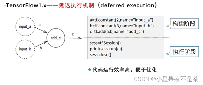
优点:代码运行效率高,便于优化
缺点:程序不够简洁;重复、冗余API
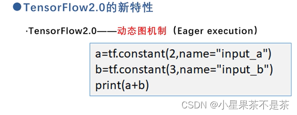
优点:能够快速的建立和调试模型;整合了重复的API,将tf.keras作为构建和训练模型的标准高级API。
缺点:执行效率不高
构架
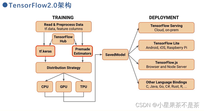
使用tf.data加载数据,feature columns描述特征,染后使用tf.keras或者Premade estimators构建训练模型,如果不想从头训练也可使用TensorFlow Hub 进行迁移学习。Distribution Strategy是一个实现分布式的API。SaveModel保存模型,保存模型后可以直接加载在程序中执行,也可以部署在服务器,嵌入式设备等中。
TensorflowDemo
tensorflow GPU安装--Tensorflow2.1-cpu安装(缺少msvcp140_1.dll)_太阳花的小绿豆的博客-CSDN博客_tensorflow2.1安装
Tensorfow
通道排序:[batch,height,width,channel]
官方demo--model代码
from tensorflow.keras.layers import Dense, Flatten, Conv2D
from tensorflow.keras import Model


class MyModel(Model):
    def __init__(self):
        super(MyModel, self).__init__()
        self.conv1 = Conv2D(32, 3, activation='relu')  # (卷积核个数,卷积核大小,步距,paddig=valid时无补零,通道数,激活函数)
        self.flatten = Flatten()  # 展平
        self.d1 = Dense(128, activation='relu')  #全连接层1 (节点个数,激活函数)
        self.d2 = Dense(10, activation='softmax')  # 全连接层2

    def call(self, x, **kwargs):  # 正向传播过程
        x = self.conv1(x)      # input[batch, 28, 28, 1] output[batch, 26, 26, 32]
        x = self.flatten(x)    # output [batch, 21632]
        x = self.d1(x)         # output [batch, 128]
        return self.d2(x)      # output [batch, 10]
padding:VALID  [向上取整]
padding:SAME  [向上取整]
1.输入图片大小W*W
2.Filter大小F* F
3.步长S
官方demo--train代码
from __future__ import absolute_import, division, print_function, unicode_literals

import tensorflow as tf
from model import MyModel


def main():
    mnist = tf.keras.datasets.mnist

    # download and load data
    (x_train, y_train), (x_test, y_test) = mnist.load_data()
    x_train, x_test = x_train / 255.0, x_test / 255.0

    # Add a channels dimension
    x_train = x_train[..., tf.newaxis]
    x_test = x_test[..., tf.newaxis]

    # create data generator
    train_ds = tf.data.Dataset.from_tensor_slices(
        (x_train, y_train)).shuffle(10000).batch(32)
    test_ds = tf.data.Dataset.from_tensor_slices((x_test, y_test)).batch(32)

    # create model
    model = MyModel()

    # define loss
    loss_object = tf.keras.losses.SparseCategoricalCrossentropy()  # 稀疏loss
    # define optimizer
    optimizer = tf.keras.optimizers.Adam()  # 优化器

    # define train_loss and train_accuracy
    train_loss = tf.keras.metrics.Mean(name='train_loss')  # 训练过程中的平均损失值
    train_accuracy = tf.keras.metrics.SparseCategoricalAccuracy(name='train_accuracy')  # 训练准确率

    # define train_loss and train_accuracy
    test_loss = tf.keras.metrics.Mean(name='test_loss')  # 测试损失值
    test_accuracy = tf.keras.metrics.SparseCategoricalAccuracy(name='test_accuracy')
  # 测试准确率
    # define train function including calculating loss, applying gradient and calculating accuracy
    @tf.function
    def train_step(images, labels):
        with tf.GradientTape() as tape:
            predictions = model(images)  # 将数据输入的模型中得到输出
            loss = loss_object(labels, predictions)  # 计算损失值
        gradients = tape.gradient(loss, model.trainable_variables)  # 将损失值反向传播到模型的每一个可训练的变量当中
        optimizer.apply_gradients(zip(gradients, model.trainable_variables))  # 将每一个节点的误差梯度用于跟新该节点的变量的值

        train_loss(loss)
        train_accuracy(labels, predictions)

    # define test function including calculating loss and calculating accuracy
    @tf.function
    def test_step(images, labels):
        predictions = model(images)
        t_loss = loss_object(labels, predictions)

        test_loss(t_loss)  # 历史损失值
        test_accuracy(labels, predictions)  # 历史准确率

    EPOCHS = 5  # 样本迭代5轮

    for epoch in range(EPOCHS):          # 每次迭代后都清空数据,否则计算就不准确了
        train_loss.reset_states()        # clear history info
        train_accuracy.reset_states()    # clear history info
        test_loss.reset_states()         # clear history info
        test_accuracy.reset_states()     # clear history info

        for images, labels in train_ds:   # 遍历训练迭代器
            train_step(images, labels)    # 计算误差等

        for test_images, test_labels in test_ds:
            test_step(test_images, test_labels)

        template = 'Epoch {}, Loss: {}, Accuracy: {}, Test Loss: {}, Test Accuracy: {}'
        print(template.format(epoch + 1,
                              train_loss.result(),
                              train_accuracy.result() * 100,
                              test_loss.result(),
                              test_accuracy.result() * 100))


if __name__ == '__main__':
    main()
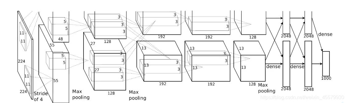
AlexNet
AlexNet是2012年ImageNet竞赛冠军获得者Hinton和他的学生Alex Krizhevsky设计的。也是在那年之后,更多的更深的神经网络被提出,比如优秀的vgg,GoogLeNet。 这对于传统的机器学习分类算法而言,已经相当的出色。
AlexNet将LeNet的思想发扬光大,把CNN的基本原理应用到了很深很宽的网络中。AlexNet主要使用到的新技术点如下:
(1)成功使用ReLU作为CNN的激活函数,并验证其效果在较深的网络超过了Sigmoid,成功解决了Sigmoid在网络较深时的梯度弥散问题。虽然ReLU激活函数在很久之前就被提出了,但是直到AlexNet的出现才将其发扬光大。
(2)训练时使用Dropout随机忽略一部分神经元,以避免模型过拟合。Dropout虽有单独的论文论述,但是AlexNet将其实用化,通过实践证实了它的效果。在AlexNet中主要是最后几个全连接层使用了Dropout。
(3)在CNN中使用重叠的最大池化。此前CNN中普遍使用平均池化,AlexNet全部使用最大池化,避免平均池化的模糊化效果。并且AlexNet中提出让步长比池化核的尺寸小,这样池化层的输出之间会有重叠和覆盖,提升了特征的丰富性。
(4)提出了LRN层,对局部神经元的活动创建竞争机制,使得其中响应比较大的值变得相对更大,并抑制其他反馈较小的神经元,增强了模型的泛化能力。
过拟合
随着训练过程的进行,模型复杂度,在training data上的error渐渐减小。可是在验证集上的error却反而渐渐增大——由于训练出来的网络过拟合了训练集,对训练集以外的数据却不work。
卷积后矩阵尺寸大小的计算
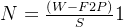
1.输入图片大小W*W
2.Filter大小F* F
3.步长S
4.padding的像素P
代码地址
tensorflow_classification/Test2_alexnet · master · mirrors / wzmiaomiao / deep-learning-for-image-processing · GitCode
model代码
from tensorflow.keras import layers, models, Model, Sequential


def AlexNet_v1(im_height=224, im_width=224, num_classes=1000):
    # tensorflow中的tensor通道排序是NHWC
    input_image = layers.Input(shape=(im_height, im_width, 3), dtype="float32")  # output(None, 224, 224, 3)
    x = layers.ZeroPadding2D(((1, 2), (1, 2)))(input_image)                      # output(None, 227, 227, 3)
    x = layers.Conv2D(48, kernel_size=11, strides=4, activation="relu")(x)       # output(None, 55, 55, 48)
    x = layers.MaxPool2D(pool_size=3, strides=2)(x)                              # output(None, 27, 27, 48)
    x = layers.Conv2D(128, kernel_size=5, padding="same", activation="relu")(x)  # output(None, 27, 27, 128)
    x = layers.MaxPool2D(pool_size=3, strides=2)(x)                              # output(None, 13, 13, 128)
    x = layers.Conv2D(192, kernel_size=3, padding="same", activation="relu")(x)  # output(None, 13, 13, 192)
    x = layers.Conv2D(192, kernel_size=3, padding="same", activation="relu")(x)  # output(None, 13, 13, 192)
    x = layers.Conv2D(128, kernel_size=3, padding="same", activation="relu")(x)  # output(None, 13, 13, 128)
    x = layers.MaxPool2D(pool_size=3, strides=2)(x)                              # output(None, 6, 6, 128)

    x = layers.Flatten()(x)                         # output(None, 6*6*128)
    x = layers.Dropout(0.2)(x)                      # 防止过拟合
    x = layers.Dense(2048, activation="relu")(x)    # output(None, 2048)
    x = layers.Dropout(0.2)(x)
    x = layers.Dense(2048, activation="relu")(x)    # output(None, 2048)
    x = layers.Dense(num_classes)(x)                  # output(None, 5)
    predict = layers.Softmax()(x)

    model = models.Model(inputs=input_image, outputs=predict)
    return model


class AlexNet_v2(Model):
    def __init__(self, num_classes=1000):
        super(AlexNet_v2, self).__init__()
        self.features = Sequential([
            layers.ZeroPadding2D(((1, 2), (1, 2))),                                 # output(None, 227, 227, 3)
            layers.Conv2D(48, kernel_size=11, strides=4, activation="relu"),        # output(None, 55, 55, 48)
            layers.MaxPool2D(pool_size=3, strides=2),                               # output(None, 27, 27, 48)
            layers.Conv2D(128, kernel_size=5, padding="same", activation="relu"),   # output(None, 27, 27, 128)
            layers.MaxPool2D(pool_size=3, strides=2),                               # output(None, 13, 13, 128)
            layers.Conv2D(192, kernel_size=3, padding="same", activation="relu"),   # output(None, 13, 13, 192)
            layers.Conv2D(192, kernel_size=3, padding="same", activation="relu"),   # output(None, 13, 13, 192)
            layers.Conv2D(128, kernel_size=3, padding="same", activation="relu"),   # output(None, 13, 13, 128)
            layers.MaxPool2D(pool_size=3, strides=2)])                              # output(None, 6, 6, 128)

        self.flatten = layers.Flatten()
        self.classifier = Sequential([
            layers.Dropout(0.2),
            layers.Dense(1024, activation="relu"),                                  # output(None, 2048)
            layers.Dropout(0.2),
            layers.Dense(128, activation="relu"),                                   # output(None, 2048)
            layers.Dense(num_classes),                                                # output(None, 5)
            layers.Softmax()
        ])

    def call(self, inputs, **kwargs):
        x = self.features(inputs)
        x = self.flatten(x)
        x = self.classifier(x)
        return x
train代码
from tensorflow.keras.preprocessing.image import ImageDataGenerator
import matplotlib.pyplot as plt
from model import AlexNet_v1, AlexNet_v2
import tensorflow as tf
import json
import os


def main():
    data_root = os.path.abspath(os.path.join(os.getcwd(), "../.."))  # get data root path
    image_path = os.path.join(data_root, "data_set", "flower_data")  # flower data set path
    train_dir = os.path.join(image_path, "train")
    validation_dir = os.path.join(image_path, "val")
    assert os.path.exists(train_dir), "cannot find {}".format(train_dir)
    assert os.path.exists(validation_dir), "cannot find {}".format(validation_dir)

    # create direction for saving weights
    if not os.path.exists("save_weights"):
        os.makedirs("save_weights")

    im_height = 224
    im_width = 224
    batch_size = 32
    epochs = 10

    # data generator with data augmentation
    train_image_generator = ImageDataGenerator(rescale=1. / 255,
                                               horizontal_flip=True)   #图像生成器,对图像进行预处理
    validation_image_generator = ImageDataGenerator(rescale=1. / 255)

    train_data_gen = train_image_generator.flow_from_directory(directory=train_dir,
                                                               batch_size=batch_size,
                                                               shuffle=True,
                                                               target_size=(im_height, im_width),
                                                               class_mode='categorical')
    total_train = train_data_gen.n  # 获得训练集样本总数

    # get class dict
    class_indices = train_data_gen.class_indices

    # transform value and key of dict
    inverse_dict = dict((val, key) for key, val in class_indices.items())
    # write dict into json file
    json_str = json.dumps(inverse_dict, indent=4)
    with open('class_indices.json', 'w') as json_file:
        json_file.write(json_str)

    val_data_gen = validation_image_generator.flow_from_directory(directory=validation_dir,
                                                                  batch_size=batch_size,
                                                                  shuffle=False,
                                                                  target_size=(im_height, im_width),
                                                                  class_mode='categorical')
    total_val = val_data_gen.n
    print("using {} images for training, {} images for validation.".format(total_train,
                                                                           total_val))

    # sample_training_images, sample_training_labels = next(train_data_gen)  # label is one-hot coding
    #
    # # This function will plot images in the form of a grid with 1 row
    # # and 5 columns where images are placed in each column.
    # def plotImages(images_arr):
    #     fig, axes = plt.subplots(1, 5, figsize=(20, 20))
    #     axes = axes.flatten()
    #     for img, ax in zip(images_arr, axes):
    #         ax.imshow(img)
    #         ax.axis('off')
    #     plt.tight_layout()
    #     plt.show()
    #
    #
    # plotImages(sample_training_images[:5])

    model = AlexNet_v1(im_height=im_height, im_width=im_width, num_classes=5)
    # model = AlexNet_v2(class_num=5)
    # model.build((batch_size, 224, 224, 3))  # when using subclass model
    model.summary()  # 模型参数信息

    # using keras high level api for training
    model.compile(optimizer=tf.keras.optimizers.Adam(learning_rate=0.0005),
                  loss=tf.keras.losses.CategoricalCrossentropy(from_logits=False),
                  metrics=["accuracy"])

    # 回调函数:控制模型训练过程中保存模型的一些参数
    callbacks = [tf.keras.callbacks.ModelCheckpoint(filepath='./save_weights/myAlex.h5',
                                                    save_best_only=True,
                                                    save_weights_only=True,
                                                    monitor='val_loss')]

    # tensorflow2.1 recommend to using fit 训练信息保存到history
    history = model.fit(x=train_data_gen,
                        steps_per_epoch=total_train // batch_size,
                        epochs=epochs,
                        validation_data=val_data_gen,
                        validation_steps=total_val // batch_size,
                        callbacks=callbacks)

    # plot loss and accuracy image
    history_dict = history.history
    train_loss = history_dict["loss"]
    train_accuracy = history_dict["accuracy"]
    val_loss = history_dict["val_loss"]
    val_accuracy = history_dict["val_accuracy"]

    # figure 1
    plt.figure()
    plt.plot(range(epochs), train_loss, label='train_loss')
    plt.plot(range(epochs), val_loss, label='val_loss')
    plt.legend()
    plt.xlabel('epochs')
    plt.ylabel('loss')

    # figure 2
    plt.figure()
    plt.plot(range(epochs), train_accuracy, label='train_accuracy')
    plt.plot(range(epochs), val_accuracy, label='val_accuracy')
    plt.legend()
    plt.xlabel('epochs')
    plt.ylabel('accuracy')
    plt.show()

    # history = model.fit_generator(generator=train_data_gen,
    #                               steps_per_epoch=total_train // batch_size,
    #                               epochs=epochs,
    #                               validation_data=val_data_gen,
    #                               validation_steps=total_val // batch_size,
    #                               callbacks=callbacks)

    # # using keras low level api for training
    # loss_object = tf.keras.losses.CategoricalCrossentropy(from_logits=False)
    # optimizer = tf.keras.optimizers.Adam(learning_rate=0.0005)
    #
    # train_loss = tf.keras.metrics.Mean(name='train_loss')
    # train_accuracy = tf.keras.metrics.CategoricalAccuracy(name='train_accuracy')
    #
    # test_loss = tf.keras.metrics.Mean(name='test_loss')
    # test_accuracy = tf.keras.metrics.CategoricalAccuracy(name='test_accuracy')
    #
    #
    # @tf.function
    # def train_step(images, labels):
    #     with tf.GradientTape() as tape:
    #         predictions = model(images, training=True)
    #         loss = loss_object(labels, predictions)
    #     gradients = tape.gradient(loss, model.trainable_variables)
    #     optimizer.apply_gradients(zip(gradients, model.trainable_variables))
    #
    #     train_loss(loss)
    #     train_accuracy(labels, predictions)
    #
    #
    # @tf.function
    # def test_step(images, labels):
    #     predictions = model(images, training=False)
    #     t_loss = loss_object(labels, predictions)
    #
    #     test_loss(t_loss)
    #     test_accuracy(labels, predictions)
    #
    #
    # best_test_loss = float('inf')
    # for epoch in range(1, epochs+1):
    #     train_loss.reset_states()        # clear history info
    #     train_accuracy.reset_states()    # clear history info
    #     test_loss.reset_states()         # clear history info
    #     test_accuracy.reset_states()     # clear history info
    #     for step in range(total_train // batch_size):
    #         images, labels = next(train_data_gen)
    #         train_step(images, labels)
    #
    #     for step in range(total_val // batch_size):
    #         test_images, test_labels = next(val_data_gen)
    #         test_step(test_images, test_labels)
    #
    #     template = 'Epoch {}, Loss: {}, Accuracy: {}, Test Loss: {}, Test Accuracy: {}'
    #     print(template.format(epoch,
    #                           train_loss.result(),
    #                           train_accuracy.result() * 100,
    #                           test_loss.result(),
    #                           test_accuracy.result() * 100))
    #     if test_loss.result() < best_test_loss:
    #        model.save_weights("./save_weights/myAlex.ckpt", save_format='tf')


if __name__ == '__main__':
    main()
predict代码
import os
import json

from PIL import Image
import numpy as np
import matplotlib.pyplot as plt

from model import AlexNet_v1, AlexNet_v2


def main():
    im_height = 224
    im_width = 224

    # load image
    img_path = "../tulip.jpg"
    assert os.path.exists(img_path), "file: '{}' dose not exist.".format(img_path)
    img = Image.open(img_path)

    # resize image to 224x224
    img = img.resize((im_width, im_height))
    plt.imshow(img)

    # scaling pixel value to (0-1)
    img = np.array(img) / 255.

    # Add the image to a batch where it's the only member.
    img = (np.expand_dims(img, 0))

    # read class_indict
    json_path = './class_indices.json'
    assert os.path.exists(json_path), "file: '{}' dose not exist.".format(json_path)

    with open(json_path, "r") as f:
        class_indict = json.load(f)

    # create model
    model = AlexNet_v1(num_classes=5)
    weighs_path = "./save_weights/myAlex.h5"
    assert os.path.exists(img_path), "file: '{}' dose not exist.".format(weighs_path)
    model.load_weights(weighs_path)

    # prediction
    result = np.squeeze(model.predict(img))
    predict_class = np.argmax(result)

    print_res = "class: {}   prob: {:.3}".format(class_indict[str(predict_class)],
                                                 result[predict_class])
    plt.title(print_res)
    for i in range(len(result)):
        print("class: {:10}   prob: {:.3}".format(class_indict[str(i)],
                                                  result[i]))
    plt.show()


if __name__ == '__main__':
    main()
VGG
文章地址:https://arxiv.org/abs/1409.1556
网络中的亮点:
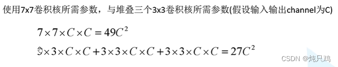
通过堆叠多个3*3的卷积核来替代大尺度卷积核(减少所需参数)-----论文中提到可通过两个3*3的卷积核来替代5*5的卷积核,堆叠三个3*3的卷积核替代7*7的卷积核。即拥有相同的感受野。
感受野
在卷积神经网络中,感受野(Receptive Field)的定义是卷积神经网络每一层输出的特征图(feature map)上的像素点在输入图片上映射的区域大小。再通俗点的解释是,特征图上的一个点对应输入图上的区域,如图所示。
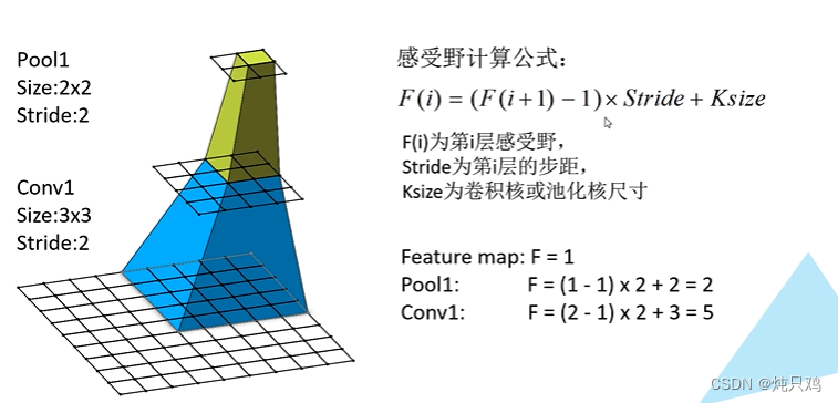
(1)注意:
1、感受野大小的计算方式是从最后一层feature map开始,往下往上的计算方法,即先计算最深层在前一层上的感受野,然后以此类推逐层传递到第一层。
2、感受野大小的计算不考虑padding的大小;
3、最后一层的特征图感受野的大小等于其卷积核的大小;
4、第i层特征图的感受野大小和第i层的卷积核大小和步长有关系,同时也与第(i+1)层特征图的感受野大小有关。
(2)感受野的作用:
1、小尺寸的卷积代替大尺寸的卷积,可减少网络参数、增加网络深度、扩大感受野,网络深度越深感受野越大性能越好;例如堆叠三个3*3卷积核与一个7*7卷积核参数的对比:
2、对于分类任务来说,最后一层特征图的感受野大小要大于等于输入图像大小,否则分类性能会不理想;
3、对于目标检测任务来说,若感受野很小,目标尺寸很大,或者目标尺寸很小,感受野很大,模型收敛困难,会严重影响检测性能;所以一般检测网络anchor的大小的获取都要依赖不同层的特征图,因为不同层次的特征图,其感受野大小不同,这样检测网络才会适应不同尺寸的目标。
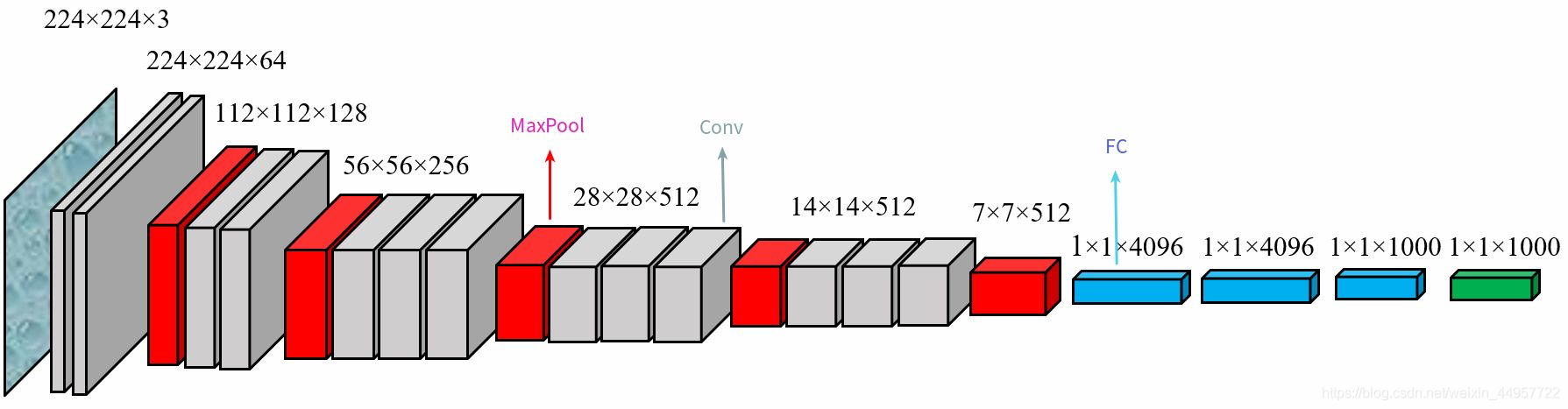
网络结构
VGGNet以下6种不同结构,我们以通常所说的VGG-16(即下图D列)为例。
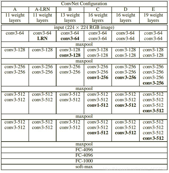
那么对于VGG16 来讲他的网络结构款加图就应该是下面这样的:
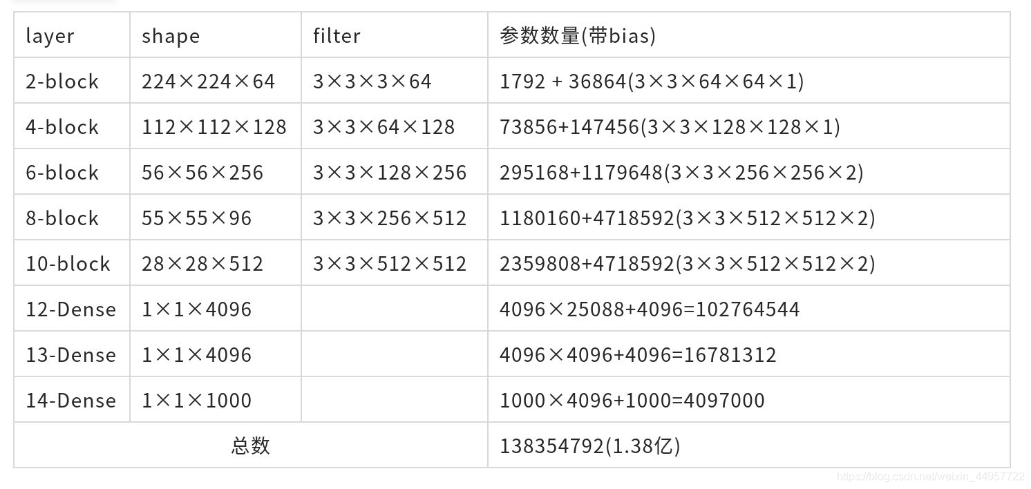
参数计算:
代码地址
deep-learning-for-image-processing/tensorflow_classification/Test3_vgg at master · WZMIAOMIAO/deep-learning-for-image-processing · GitHub
model代码
from tensorflow.keras import layers, Model, Sequential

CONV_KERNEL_INITIALIZER = {
    'class_name': 'VarianceScaling',
    'config': {
        'scale': 2.0,
        'mode': 'fan_out',
        'distribution': 'truncated_normal'
    }
}

DENSE_KERNEL_INITIALIZER = {
    'class_name': 'VarianceScaling',
    'config': {
        'scale': 1. / 3.,
        'mode': 'fan_out',
        'distribution': 'uniform'
    }
}

# 特征分类网络
def VGG(feature, im_height=224, im_width=224, num_classes=1000):
    # tensorflow中的tensor通道排序是NHWC
    input_image = layers.Input(shape=(im_height, im_width, 3), dtype="float32")
    x = feature(input_image)
    x = layers.Flatten()(x)
    x = layers.Dropout(rate=0.5)(x)
    x = layers.Dense(4096, activation='relu',
                     kernel_initializer=DENSE_KERNEL_INITIALIZER)(x)
    x = layers.Dropout(rate=0.5)(x)
    x = layers.Dense(4096, activation='relu',
                     kernel_initializer=DENSE_KERNEL_INITIALIZER)(x)
    x = layers.Dense(num_classes,
                     kernel_initializer=DENSE_KERNEL_INITIALIZER)(x)
    output = layers.Softmax()(x)
    model = Model(inputs=input_image, outputs=output)
    return model

# 特征提取网络
def make_feature(cfg):
    feature_layers = []
    for v in cfg:
        if v == "M":
            feature_layers.append(layers.MaxPool2D(pool_size=2, strides=2))
        else:
            conv2d = layers.Conv2D(v, kernel_size=3, padding="SAME", activation="relu",
                                   kernel_initializer=CONV_KERNEL_INITIALIZER)
            feature_layers.append(conv2d)
    return Sequential(feature_layers, name="feature")

# 配置列表
cfgs = {
    'vgg11': [64, 'M', 128, 'M', 256, 256, 'M', 512, 512, 'M', 512, 512, 'M'],
    'vgg13': [64, 64, 'M', 128, 128, 'M', 256, 256, 'M', 512, 512, 'M', 512, 512, 'M'],
    'vgg16': [64, 64, 'M', 128, 128, 'M', 256, 256, 256, 'M', 512, 512, 512, 'M', 512, 512, 512, 'M'],
    'vgg19': [64, 64, 'M', 128, 128, 'M', 256, 256, 256, 256, 'M', 512, 512, 512, 512, 'M', 512, 512, 512, 512, 'M'],
}


def vgg(model_name="vgg16", im_height=224, im_width=224, num_classes=1000):
    assert model_name in cfgs.keys(), "not support model {}".format(model_name)
    cfg = cfgs[model_name]
    model = VGG(make_feature(cfg), im_height=im_height, im_width=im_width, num_classes=num_classes)
    return model
train代码
from tensorflow.keras.preprocessing.image import ImageDataGenerator
import matplotlib.pyplot as plt
from model import vgg
import tensorflow as tf
import json
import os


def main():
    data_root = os.path.abspath(os.path.join(os.getcwd(), "../.."))  # get data root path
    image_path = os.path.join(data_root, "data_set", "flower_data")  # flower data set path
    train_dir = os.path.join(image_path, "train")
    validation_dir = os.path.join(image_path, "val")
    assert os.path.exists(train_dir), "cannot find {}".format(train_dir)
    assert os.path.exists(validation_dir), "cannot find {}".format(validation_dir)

    # create direction for saving weights
    if not os.path.exists("save_weights"):
        os.makedirs("save_weights")

    im_height = 224
    im_width = 224
    batch_size = 32
    epochs = 10

    # data generator with data augmentation
    train_image_generator = ImageDataGenerator(rescale=1. / 255,
                                               horizontal_flip=True)
    validation_image_generator = ImageDataGenerator(rescale=1. / 255)

    train_data_gen = train_image_generator.flow_from_directory(directory=train_dir,
                                                               batch_size=batch_size,
                                                               shuffle=True,
                                                               target_size=(im_height, im_width),
                                                               class_mode='categorical')
    total_train = train_data_gen.n

    # get class dict
    class_indices = train_data_gen.class_indices

    # transform value and key of dict
    inverse_dict = dict((val, key) for key, val in class_indices.items())
    # write dict into json file
    json_str = json.dumps(inverse_dict, indent=4)
    with open('class_indices.json', 'w') as json_file:
        json_file.write(json_str)

    val_data_gen = validation_image_generator.flow_from_directory(directory=validation_dir,
                                                                  batch_size=batch_size,
                                                                  shuffle=False,
                                                                  target_size=(im_height, im_width),
                                                                  class_mode='categorical')
    total_val = val_data_gen.n
    print("using {} images for training, {} images for validation.".format(total_train,
                                                                           total_val))

    model = vgg("vgg16", im_height, im_width, num_classes=5)
    model.summary()

    # using keras high level api for training
    model.compile(optimizer=tf.keras.optimizers.Adam(learning_rate=0.0001),
                  loss=tf.keras.losses.CategoricalCrossentropy(from_logits=False),
                  metrics=["accuracy"])

    callbacks = [tf.keras.callbacks.ModelCheckpoint(filepath='./save_weights/myVGG.h5',
                                                    save_best_only=True,
                                                    save_weights_only=True,
                                                    monitor='val_loss')]

    # tensorflow2.1 recommend to using fit
    history = model.fit(x=train_data_gen,
                        steps_per_epoch=total_train // batch_size,
                        epochs=epochs,
                        validation_data=val_data_gen,
                        validation_steps=total_val // batch_size,
                        callbacks=callbacks)

    # plot loss and accuracy image
    history_dict = history.history
    train_loss = history_dict["loss"]
    train_accuracy = history_dict["accuracy"]
    val_loss = history_dict["val_loss"]
    val_accuracy = history_dict["val_accuracy"]

    # figure 1
    plt.figure()
    plt.plot(range(epochs), train_loss, label='train_loss')
    plt.plot(range(epochs), val_loss, label='val_loss')
    plt.legend()
    plt.xlabel('epochs')
    plt.ylabel('loss')

    # figure 2
    plt.figure()
    plt.plot(range(epochs), train_accuracy, label='train_accuracy')
    plt.plot(range(epochs), val_accuracy, label='val_accuracy')
    plt.legend()
    plt.xlabel('epochs')
    plt.ylabel('accuracy')
    plt.show()


if __name__ == '__main__':
    main()
GoogLeNet
论文地址:https://arxiv.org/pdf/1409.4842.pdf
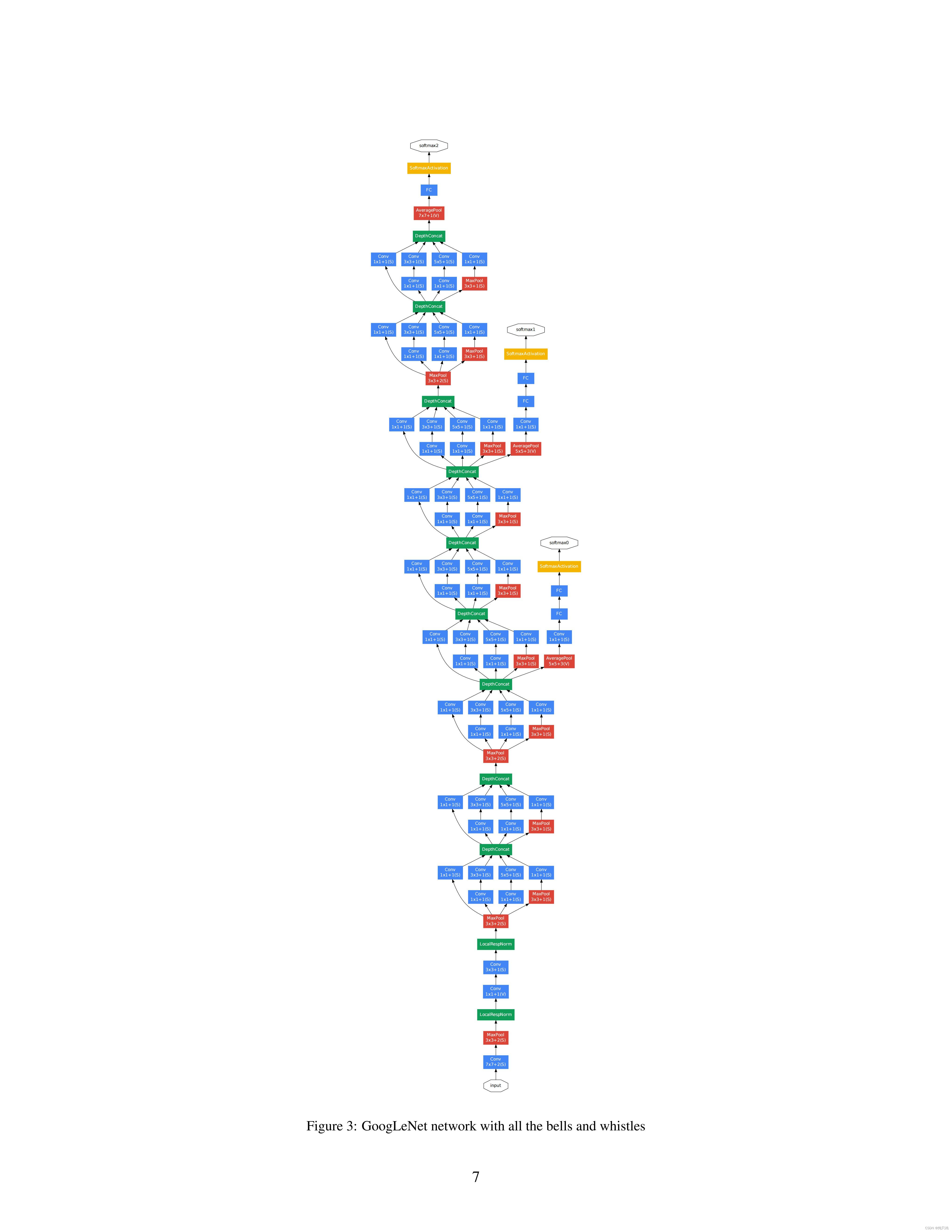
GoogLeNet网络的主要创新点在于:
1.提出Inception结构(融合不同尺寸的特征信息);
2.使用1X1的卷积进行降维以及映射处理;
3.添加两个辅助分类器帮助训练;
4.丢弃全连接层,使用平均池化层(大大减少模型参数)。
AlexNet和VGG都只有一个输出层GoogLeNet有三个输出层(其中两个辅助分类层)。
GoogLeNet网络结构
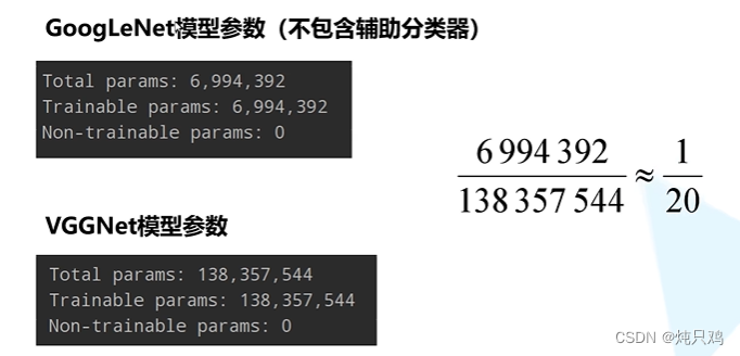
参数
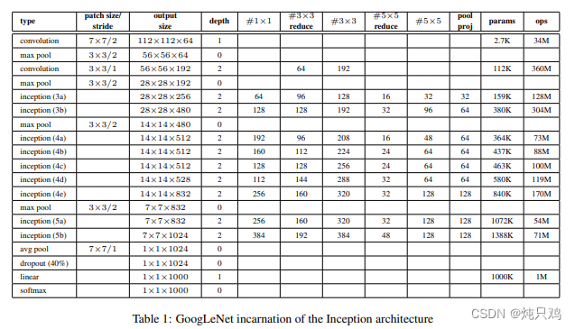
GoogleNet与VGG参数对比:
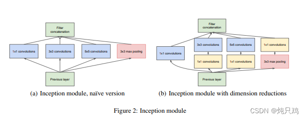
Inception结构
1*1的卷积操作的目的是减少特征矩阵的深度,从而减少特征参数
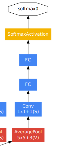
辅助分类器结构
代码地址
deep-learning-for-image-processing/tensorflow_classification/Test4_goolenet at master · WZMIAOMIAO/deep-learning-for-image-processing · GitHub
model代码
from tensorflow.keras import layers, models, Model, Sequential


def GoogLeNet(im_height=224, im_width=224, class_num=1000, aux_logits=False):
    # tensorflow中的tensor通道排序是NHWC
    input_image = layers.Input(shape=(im_height, im_width, 3), dtype="float32")
    # (None, 224, 224, 3)
    x = layers.Conv2D(64, kernel_size=7, strides=2, padding="SAME", activation="relu", name="conv2d_1")(input_image)
    # (None, 112, 112, 64)
    x = layers.MaxPool2D(pool_size=3, strides=2, padding="SAME", name="maxpool_1")(x)
    # (None, 56, 56, 64)
    x = layers.Conv2D(64, kernel_size=1, activation="relu", name="conv2d_2")(x)
    # (None, 56, 56, 64)
    x = layers.Conv2D(192, kernel_size=3, padding="SAME", activation="relu", name="conv2d_3")(x)
    # (None, 56, 56, 192)
    x = layers.MaxPool2D(pool_size=3, strides=2, padding="SAME", name="maxpool_2")(x)

    # (None, 28, 28, 192)
    x = Inception(64, 96, 128, 16, 32, 32, name="inception_3a")(x)
    # (None, 28, 28, 256)
    x = Inception(128, 128, 192, 32, 96, 64, name="inception_3b")(x)

    # (None, 28, 28, 480)
    x = layers.MaxPool2D(pool_size=3, strides=2, padding="SAME", name="maxpool_3")(x)
    # (None, 14, 14, 480)
    x = Inception(192, 96, 208, 16, 48, 64, name="inception_4a")(x)
    if aux_logits:
        aux1 = InceptionAux(class_num, name="aux_1")(x)

    # (None, 14, 14, 512)
    x = Inception(160, 112, 224, 24, 64, 64, name="inception_4b")(x)
    # (None, 14, 14, 512)
    x = Inception(128, 128, 256, 24, 64, 64, name="inception_4c")(x)
    # (None, 14, 14, 512)
    x = Inception(112, 144, 288, 32, 64, 64, name="inception_4d")(x)
    if aux_logits:
        aux2 = InceptionAux(class_num, name="aux_2")(x)

    # (None, 14, 14, 528)
    x = Inception(256, 160, 320, 32, 128, 128, name="inception_4e")(x)
    # (None, 14, 14, 532)
    x = layers.MaxPool2D(pool_size=3, strides=2, padding="SAME", name="maxpool_4")(x)

    # (None, 7, 7, 832)
    x = Inception(256, 160, 320, 32, 128, 128, name="inception_5a")(x)
    # (None, 7, 7, 832)
    x = Inception(384, 192, 384, 48, 128, 128, name="inception_5b")(x)
    # (None, 7, 7, 1024)
    x = layers.AvgPool2D(pool_size=7, strides=1, name="avgpool_1")(x)

    # (None, 1, 1, 1024)
    x = layers.Flatten(name="output_flatten")(x)
    # (None, 1024)
    x = layers.Dropout(rate=0.4, name="output_dropout")(x)
    x = layers.Dense(class_num, name="output_dense")(x)
    # (None, class_num)
    aux3 = layers.Softmax(name="aux_3")(x)

    if aux_logits:
        model = models.Model(inputs=input_image, outputs=[aux1, aux2, aux3])
    else:
        model = models.Model(inputs=input_image, outputs=aux3)
    return model


class Inception(layers.Layer):
    def __init__(self, ch1x1, ch3x3red, ch3x3, ch5x5red, ch5x5, pool_proj, **kwargs):
        super(Inception, self).__init__(**kwargs)
        self.branch1 = layers.Conv2D(ch1x1, kernel_size=1, activation="relu")

        self.branch2 = Sequential([
            layers.Conv2D(ch3x3red, kernel_size=1, activation="relu"),
            layers.Conv2D(ch3x3, kernel_size=3, padding="SAME", activation="relu")])      # output_size= input_size

        self.branch3 = Sequential([
            layers.Conv2D(ch5x5red, kernel_size=1, activation="relu"),
            layers.Conv2D(ch5x5, kernel_size=5, padding="SAME", activation="relu")])      # output_size= input_size

        self.branch4 = Sequential([
            layers.MaxPool2D(pool_size=3, strides=1, padding="SAME"),  # caution: default strides==pool_size
            layers.Conv2D(pool_proj, kernel_size=1, activation="relu")])                  # output_size= input_size

  #正向传播
    def call(self, inputs, **kwargs):
        branch1 = self.branch1(inputs)
        branch2 = self.branch2(inputs)
        branch3 = self.branch3(inputs)
        branch4 = self.branch4(inputs)
        outputs = layers.concatenate([branch1, branch2, branch3, branch4])  # 通过concatenate函数在深度方向进行拼接
        return outputs

# 辅助分类器
class InceptionAux(layers.Layer):
    def __init__(self, num_classes, **kwargs):
        super(InceptionAux, self).__init__(**kwargs)
        self.averagePool = layers.AvgPool2D(pool_size=5, strides=3)
        self.conv = layers.Conv2D(128, kernel_size=1, activation="relu")

        self.fc1 = layers.Dense(1024, activation="relu")
        self.fc2 = layers.Dense(num_classes)
        self.softmax = layers.Softmax()

  # 正向传播
    def call(self, inputs, **kwargs):
        # aux1: N x 512 x 14 x 14, aux2: N x 528 x 14 x 14
        x = self.averagePool(inputs)
        # aux1: N x 512 x 4 x 4, aux2: N x 528 x 4 x 4
        x = self.conv(x)
        # N x 128 x 4 x 4
        x = layers.Flatten()(x)
        x = layers.Dropout(rate=0.5)(x)
        # N x 2048
        x = self.fc1(x)
        x = layers.Dropout(rate=0.5)(x)
        # N x 1024
        x = self.fc2(x)
        # N x num_classes
        x = self.softmax(x)

        return x
ResNet
文章地址:https://arxiv.org/abs/1512.03385
网络中的亮点:
1.超深的网络结构(超过1000层)。
2.提出residual(残差结构)模块。
3.使用Batch Normalization 加速训练(丢弃dropout)。
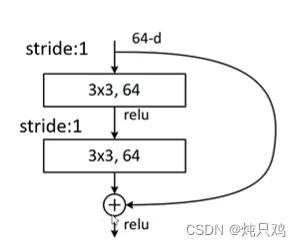
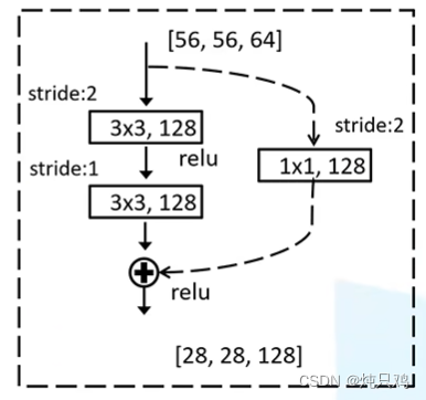
residual结构
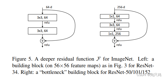
参数:
L:3*3*64*64+3*3*64*64=73,728
R:1*1*256*64+3*3*64*64+1*1*64*256=69,632
注意:主分支与shortcut的输出的矩阵shape必须相同。
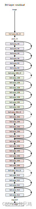
34层残差结构
参数表
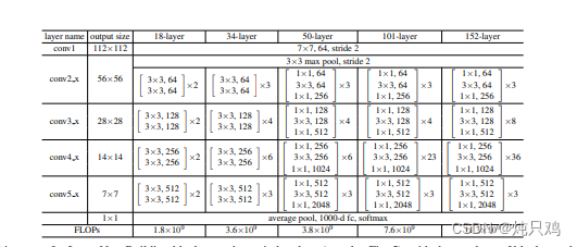
实线残差结构:
输入shape和输出shape一模一样
虚线残差结构:
输入的shape和输出的shape不一样
Batch Normalization
Batch Normalization详解以及pytorch实验_太阳花的小绿豆的博客-CSDN博客_batch normalization pytorch
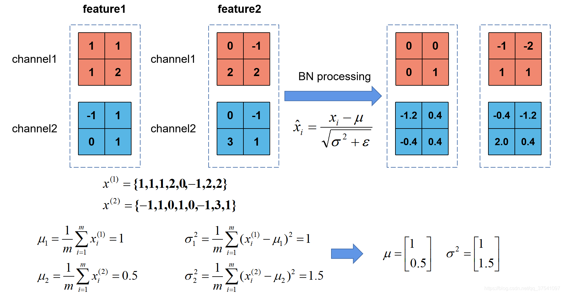
Batch Normalization的目的是使我们的一批(Batch)feature map满足均值为0,方差为1的分布律。
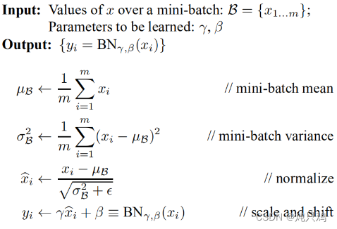
 和
和 是通过反向传播学习得到的
例如
 是一个很小的数,防止分母为零。
使用BN时需要注意的问题
(1)训练时要将traning参数设置为True,在验证时将trainning参数设置为False。在pytorch中可通过创建模型的model.train()和model.eval()方法控制。
(2)batch size尽可能设置大点,设置小后表现可能很糟糕,设置的越大求的均值和方差越接近整个训练集的均值和方差。
(3)建议将bn层放在卷积层(Conv)和激活层(例如Relu)之间,且卷积层不要使用偏置bias,因为没有用。
迁移学习
使用迁移学习的优势:
1.能够快速的训练出一个理想的结果。
2.当数据集较小时也能训练出理想的效果。
注意:用别人的模型时要注意他的预处理方式。
常见的迁移学习方式:
1.载入权重后训练所有参数。
2.载入权重后只训练最后几层参数。
3.载入权重后在原网络基础上再添加一层全连接层,仅训练最后一个全连接层。
ResNeXt
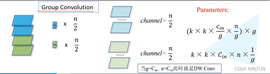
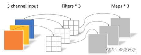
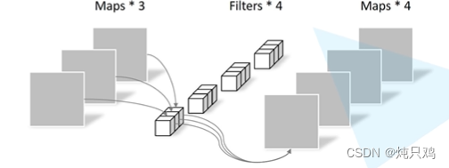
组卷积操作
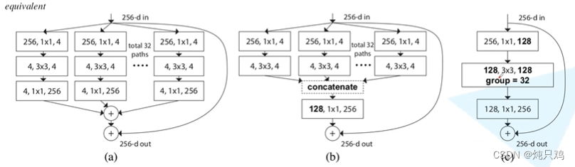
ResNeXt的block
下面三个block模块,它们在数学计算上是等价的。
与ResNet对比
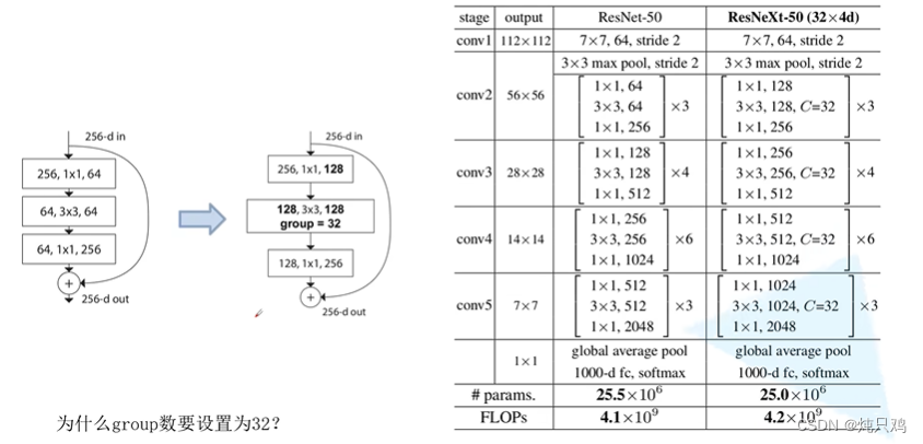
C=32时错误率低
代码地址
deep-learning-for-image-processing/tensorflow_classification/Test5_resnet at master · WZMIAOMIAO/deep-learning-for-image-processing · GitHub
model
from tensorflow.keras import layers, Model, Sequential


class BasicBlock(layers.Layer):
    expansion = 1  # 残差结构中卷积核变化系数

    def __init__(self, out_channel, strides=1, downsample=None, **kwargs):  # dpwnsample是下采样
        super(BasicBlock, self).__init__(**kwargs)
        self.conv1 = layers.Conv2D(out_channel, kernel_size=3, strides=strides,
                                   padding="SAME", use_bias=False)
        self.bn1 = layers.BatchNormalization(momentum=0.9, epsilon=1e-5)
        # -----------------------------------------
        self.conv2 = layers.Conv2D(out_channel, kernel_size=3, strides=1,
                                   padding="SAME", use_bias=False)
        self.bn2 = layers.BatchNormalization(momentum=0.9, epsilon=1e-5)
        # -----------------------------------------
        self.downsample = downsample
        self.relu = layers.ReLU()
        self.add = layers.Add()

    def call(self, inputs, training=False):
        identity = inputs
        if self.downsample is not None:
            identity = self.downsample(inputs)

        x = self.conv1(inputs)
        x = self.bn1(x, training=training)
        x = self.relu(x)

        x = self.conv2(x)
        x = self.bn2(x, training=training)

        x = self.add([identity, x])
        x = self.relu(x)

        return x


class Bottleneck(layers.Layer):
    """
    注意:原论文中,在虚线残差结构的主分支上,第一个1x1卷积层的步距是2,第二个3x3卷积层步距是1。
    但在pytorch官方实现过程中是第一个1x1卷积层的步距是1,第二个3x3卷积层步距是2,
    这么做的好处是能够在top1上提升大概0.5%的准确率。
    可参考Resnet v1.5 https://ngc.nvidia.com/catalog/model-scripts/nvidia:resnet_50_v1_5_for_pytorch
    """
    expansion = 4

    def __init__(self, out_channel, strides=1, downsample=None, **kwargs):
        super(Bottleneck, self).__init__(**kwargs)
        self.conv1 = layers.Conv2D(out_channel, kernel_size=1, use_bias=False, name="conv1")
        self.bn1 = layers.BatchNormalization(momentum=0.9, epsilon=1e-5, name="conv1/BatchNorm")
        # -----------------------------------------
        self.conv2 = layers.Conv2D(out_channel, kernel_size=3, use_bias=False,
                                   strides=strides, padding="SAME", name="conv2")
        self.bn2 = layers.BatchNormalization(momentum=0.9, epsilon=1e-5, name="conv2/BatchNorm")
        # -----------------------------------------
        self.conv3 = layers.Conv2D(out_channel * self.expansion, kernel_size=1, use_bias=False, name="conv3")
        self.bn3 = layers.BatchNormalization(momentum=0.9, epsilon=1e-5, name="conv3/BatchNorm")
        # -----------------------------------------
        self.relu = layers.ReLU()
        self.downsample = downsample
        self.add = layers.Add()

    def call(self, inputs, training=False):
        identity = inputs
        if self.downsample is not None:
            identity = self.downsample(inputs)

        x = self.conv1(inputs)
        x = self.bn1(x, training=training)
        x = self.relu(x)

        x = self.conv2(x)
        x = self.bn2(x, training=training)
        x = self.relu(x)

        x = self.conv3(x)
        x = self.bn3(x, training=training)

        x = self.add([x, identity])
        x = self.relu(x)

        return x


def _make_layer(block, in_channel, channel, block_num, name, strides=1):
    downsample = None
    if strides != 1 or in_channel != channel * block.expansion:
        downsample = Sequential([
            layers.Conv2D(channel * block.expansion, kernel_size=1, strides=strides,
                          use_bias=False, name="conv1"),
            layers.BatchNormalization(momentum=0.9, epsilon=1.001e-5, name="BatchNorm")
        ], name="shortcut")

    layers_list = []
    layers_list.append(block(channel, downsample=downsample, strides=strides, name="unit_1"))

    for index in range(1, block_num):
        layers_list.append(block(channel, name="unit_" + str(index + 1)))

    return Sequential(layers_list, name=name)


#  定义resnet网络框架
def _resnet(block, blocks_num, im_width=224, im_height=224, num_classes=1000, include_top=True):
    # tensorflow中的tensor通道排序是NHWC
    # (None, 224, 224, 3)
    input_image = layers.Input(shape=(im_height, im_width, 3), dtype="float32")
    x = layers.Conv2D(filters=64, kernel_size=7, strides=2,
                      padding="SAME", use_bias=False, name="conv1")(input_image)
    x = layers.BatchNormalization(momentum=0.9, epsilon=1e-5, name="conv1/BatchNorm")(x)
    x = layers.ReLU()(x)
    x = layers.MaxPool2D(pool_size=3, strides=2, padding="SAME")(x)

    x = _make_layer(block, x.shape[-1], 64, blocks_num[0], name="block1")(x)
    x = _make_layer(block, x.shape[-1], 128, blocks_num[1], strides=2, name="block2")(x)
    x = _make_layer(block, x.shape[-1], 256, blocks_num[2], strides=2, name="block3")(x)
    x = _make_layer(block, x.shape[-1], 512, blocks_num[3], strides=2, name="block4")(x)

    if include_top:
        x = layers.GlobalAvgPool2D()(x)  # pool + flatten
        x = layers.Dense(num_classes, name="logits")(x)
        predict = layers.Softmax()(x)
    else:
        predict = x

    model = Model(inputs=input_image, outputs=predict)

    return model


def resnet34(im_width=224, im_height=224, num_classes=1000, include_top=True):
    return _resnet(BasicBlock, [3, 4, 6, 3], im_width, im_height, num_classes, include_top)


def resnet50(im_width=224, im_height=224, num_classes=1000, include_top=True):
    return _resnet(Bottleneck, [3, 4, 6, 3], im_width, im_height, num_classes, include_top)


def resnet101(im_width=224, im_height=224, num_classes=1000, include_top=True):
    return _resnet(Bottleneck, [3, 4, 23, 3], im_width, im_height, num_classes, include_top)
train代码
import os
import sys
import glob
import json

import tensorflow as tf
from tensorflow.keras.preprocessing.image import ImageDataGenerator
from tqdm import tqdm

from model import resnet50


def main():
    data_root = os.path.abspath(os.path.join(os.getcwd(), "../.."))  # get data root path
    image_path = os.path.join(data_root, "data_set", "flower_data")  # flower data set path
    train_dir = os.path.join(image_path, "train")
    validation_dir = os.path.join(image_path, "val")
    assert os.path.exists(train_dir), "cannot find {}".format(train_dir)
    assert os.path.exists(validation_dir), "cannot find {}".format(validation_dir)

    im_height = 224
    im_width = 224
    batch_size = 16
    epochs = 20
    num_classes = 5

    _R_MEAN = 123.68
    _G_MEAN = 116.78
    _B_MEAN = 103.94


    #  图像预处理
    def pre_function(img):
        # img = im.open('test.jpg')
        # img = np.array(img).astype(np.float32)
        img = img - [_R_MEAN, _G_MEAN, _B_MEAN]

        return img

    # data generator with data augmentation
    train_image_generator = ImageDataGenerator(horizontal_flip=True,
                                               preprocessing_function=pre_function)

    validation_image_generator = ImageDataGenerator(preprocessing_function=pre_function)

    train_data_gen = train_image_generator.flow_from_directory(directory=train_dir,
                                                               batch_size=batch_size,
                                                               shuffle=True,
                                                               target_size=(im_height, im_width),
                                                               class_mode='categorical')
    total_train = train_data_gen.n

    # get class dict
    class_indices = train_data_gen.class_indices

    # transform value and key of dict
    inverse_dict = dict((val, key) for key, val in class_indices.items())
    # write dict into json file
    json_str = json.dumps(inverse_dict, indent=4)
    with open('class_indices.json', 'w') as json_file:
        json_file.write(json_str)

    val_data_gen = validation_image_generator.flow_from_directory(directory=validation_dir,
                                                                  batch_size=batch_size,
                                                                  shuffle=False,
                                                                  target_size=(im_height, im_width),
                                                                  class_mode='categorical')
    # img, _ = next(train_data_gen)
    total_val = val_data_gen.n
    print("using {} images for training, {} images for validation.".format(total_train,
                                                                           total_val))

    feature = resnet50(num_classes=5, include_top=False)
    # feature.build((None, 224, 224, 3))  # when using subclass model

    # 直接下载我转好的权重
    # download weights 链接: https://pan.baidu.com/s/1tLe9ahTMIwQAX7do_S59Zg  密码: u199
    pre_weights_path = './pretrain_weights.ckpt'
    assert len(glob.glob(pre_weights_path+"*")), "cannot find {}".format(pre_weights_path)
    feature.load_weights(pre_weights_path)
    feature.trainable = False  # feature的所有权重都会被冻结,训练过程中也无法在训练这些参数,training设置为true也不行
    feature.summary()

    model = tf.keras.Sequential([feature,
                                 tf.keras.layers.GlobalAvgPool2D(),
                                 tf.keras.layers.Dropout(rate=0.5),
                                 tf.keras.layers.Dense(1024, activation="relu"),
                                 tf.keras.layers.Dropout(rate=0.5),
                                 tf.keras.layers.Dense(num_classes),
                                 tf.keras.layers.Softmax()])
    # model.build((None, 224, 224, 3))
    model.summary()

    # using keras low level api for training
    loss_object = tf.keras.losses.CategoricalCrossentropy(from_logits=False)
    optimizer = tf.keras.optimizers.Adam(learning_rate=0.0002)

    train_loss = tf.keras.metrics.Mean(name='train_loss')
    train_accuracy = tf.keras.metrics.CategoricalAccuracy(name='train_accuracy')

    val_loss = tf.keras.metrics.Mean(name='val_loss')
    val_accuracy = tf.keras.metrics.CategoricalAccuracy(name='val_accuracy')

    @tf.function
    def train_step(images, labels):
        with tf.GradientTape() as tape:
            output = model(images, training=True)
            loss = loss_object(labels, output)
        gradients = tape.gradient(loss, model.trainable_variables)
        optimizer.apply_gradients(zip(gradients, model.trainable_variables))

        train_loss(loss)
        train_accuracy(labels, output)

    @tf.function
    def val_step(images, labels):
        output = model(images, training=False)
        loss = loss_object(labels, output)

        val_loss(loss)
        val_accuracy(labels, output)

    best_val_acc = 0.
    for epoch in range(epochs):
        train_loss.reset_states()  # clear history info
        train_accuracy.reset_states()  # clear history info
        val_loss.reset_states()  # clear history info
        val_accuracy.reset_states()  # clear history info

        # train
        train_bar = tqdm(range(total_train // batch_size), file=sys.stdout)
        for step in train_bar:
            images, labels = next(train_data_gen)
            train_step(images, labels)

            # print train process
            train_bar.desc = "train epoch[{}/{}] loss:{:.3f}, acc:{:.3f}".format(epoch + 1,
                                                                                 epochs,
                                                                                 train_loss.result(),
                                                                                 train_accuracy.result())

        # validate
        val_bar = tqdm(range(total_val // batch_size), file=sys.stdout)
        for step in val_bar:
            test_images, test_labels = next(val_data_gen)
            val_step(test_images, test_labels)

            # print val process
            val_bar.desc = "valid epoch[{}/{}] loss:{:.3f}, acc:{:.3f}".format(epoch + 1,
                                                                               epochs,
                                                                               val_loss.result(),
                                                                               val_accuracy.result())

        # only save best weights
        if val_accuracy.result() > best_val_acc:
            best_val_acc = val_accuracy.result()
            model.save_weights("./save_weights/resNet_50.ckpt", save_format="tf")


if __name__ == '__main__':
    main()
MobileNet
MobileNets 基于流线型架构,使用深度可分离卷积来构建轻量级深度神经网络,用于移动和嵌入式视觉应用。该网络引入了两个简单的全局超参数——宽度乘数和分辨率乘数,可以有效地在延迟和准确性之间进行权衡。这些超参数允许模型构建者根据问题的限制条件为其应用程序选择合适大小的模型。
MobileNet v1
https://arxiv.org/abs/1704.04861
传统卷积

DW卷积(depthwise separable conv)

PW卷积(pointwise conv)
PW卷积与普通卷积的区别是卷积核的大小是1
一般DW和PW一起使用,理论上普通卷积计算量是DW+PW的8-9倍。
MobileNet v2
https://arxiv.org/abs/1801.04381
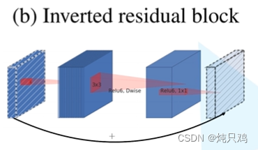
更加高效的 MobileNetV2 继续使用了 MobileNetV1 提出的深度可分离卷积(Depthwise separable convolutions),同时引入了线性瓶颈结构(Linear Bottlenecks),反向残差结构(Inverted Residuals),使得参数量和计算量减少,速度提升,精度更高。
反向残差结构
传统残差结构是一个瓶颈形结构,先降维再升维。采用relu激活函数。
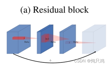
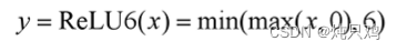
反向残差结构先升维再降维。采用relu6激活函数。
MobileNet v3
https://arxiv.org/abs/1905.02244
Self-Attention
https://arxiv.org/abs/1706.03762
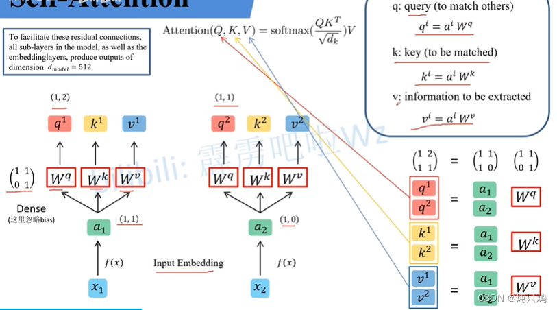
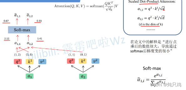
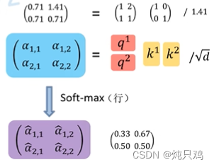
d是k的个数
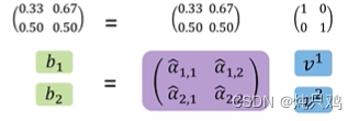
使用矩阵计算: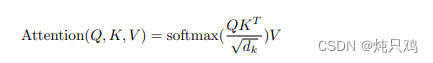
接下来对求得的 进行操作:将
 与
与 相乘,
相乘, 与
与 相乘,然后将二值相加得到
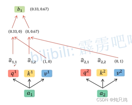
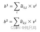
用矩阵乘法表示:
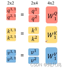
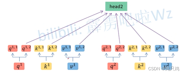
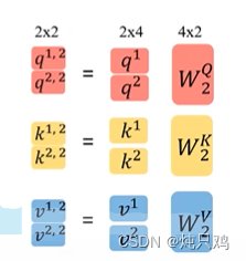
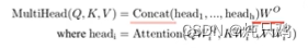
Multi-head Self-Attention
2个head的情况
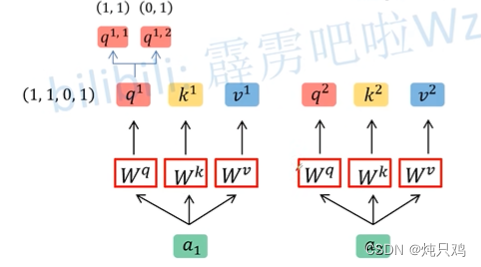
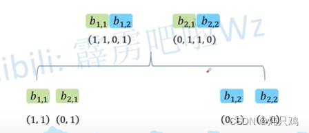
将 (1,1,0,1)按照head的个数拆分成(1,1),(0,1)。
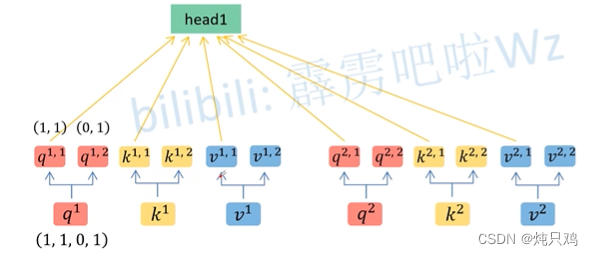
得到 和
和
得到 和
和
然后将b拼接
原文链接:Vision Transformer详解_太阳花的小绿豆的博客-CSDN博客
论文下载链接:https://arxiv.org/abs/2010.11929
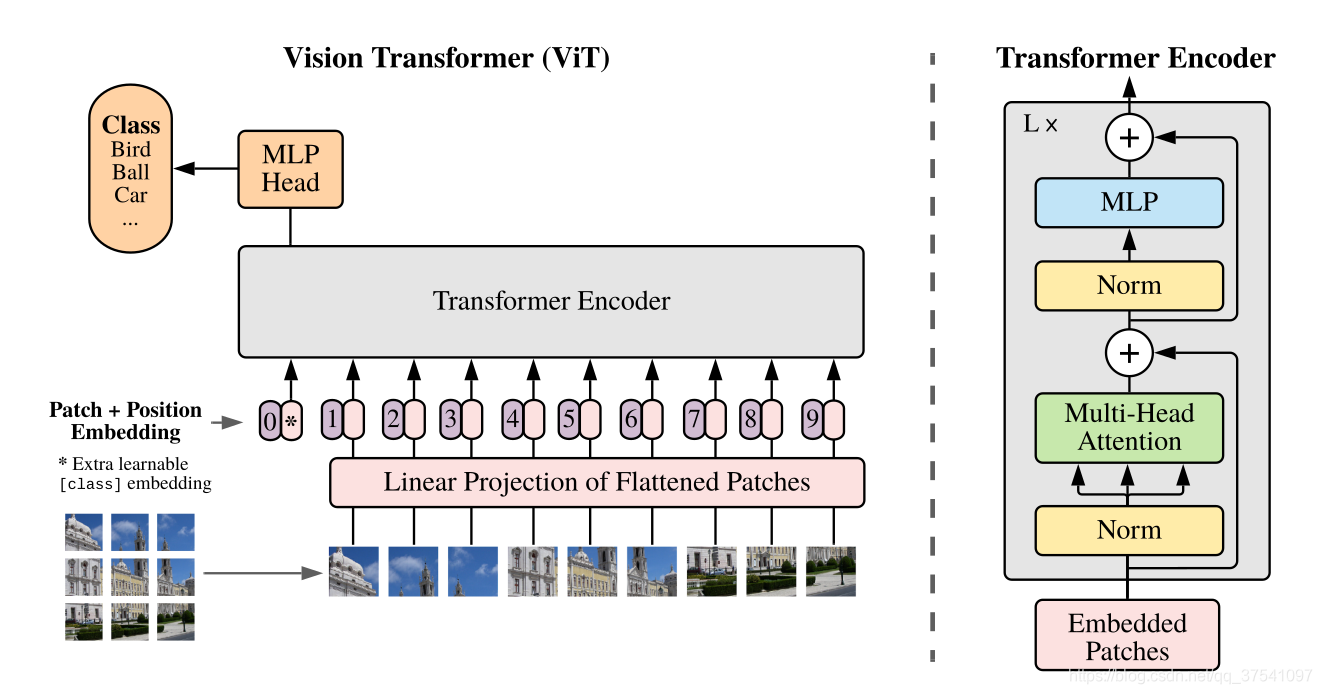
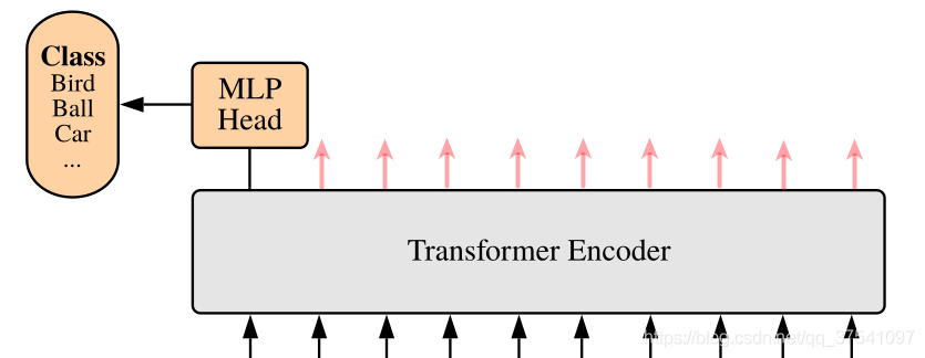
模型架构
下图是原论文中给出的关于Vision Transformer(ViT)的模型框架。模型由三个模块组成:
Linear Projection of Flattened Patches(Embedding层)
Transformer Encoder(图右侧有给出更加详细的结构)
MLP Head(最终用于分类的层结构)
动态演示:ViT的动态过程 - 知乎
Embedding层结构
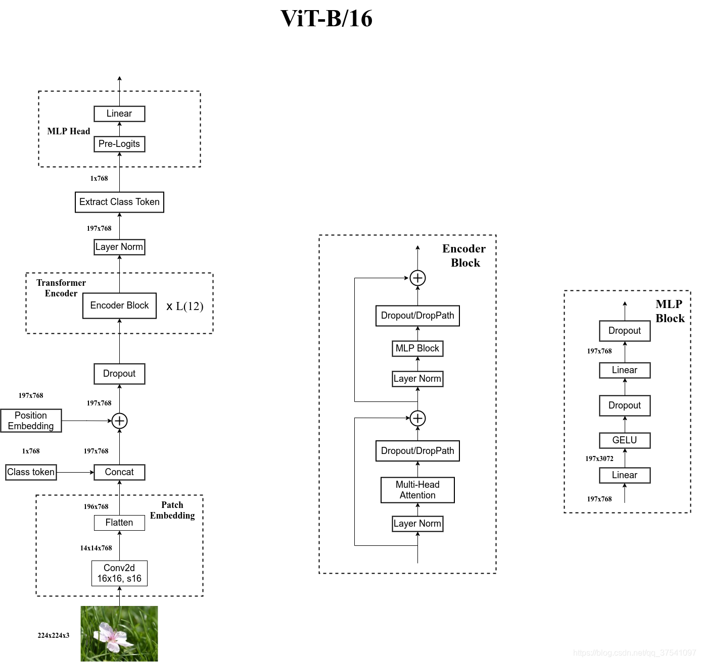
对于标准的Transformer模块,要求输入的是token(向量)序列,即二维矩阵[num_token, token_dim],如下图,token0-9对应的都是向量,以ViT-B/16为例,每个token向量长度为768。
对于图像数据而言,其数据格式为[H, W, C]是三维矩阵明显不是Transformer想要的。所以需要先通过一个Embedding层来对数据做个变换。如下图所示,首先将一张图片按给定大小分成一堆Patches。以ViT-B/16为例,将输入图片(224x224)按照16x16大小的Patch进行划分,划分后会得到(224/16)^2 =196个Patches。接着通过线性映射将每个Patch映射到一维向量中,以ViT-B/16为例,每个Patche数据shape为[16, 16, 3]通过映射得到一个长度为768的向量(后面都直接称为token)。[16, 16, 3] -> [768]
在代码实现中,直接通过一个卷积层来实现。 以ViT-B/16为例,直接使用一个卷积核大小为16x16,步距为16,卷积核个数为768的卷积来实现。通过卷积[224, 224, 3] -> [14, 14, 768],然后把H以及W两个维度展平即可[14, 14, 768] -> [196, 768],此时正好变成了一个二维矩阵,正是Transformer想要的。
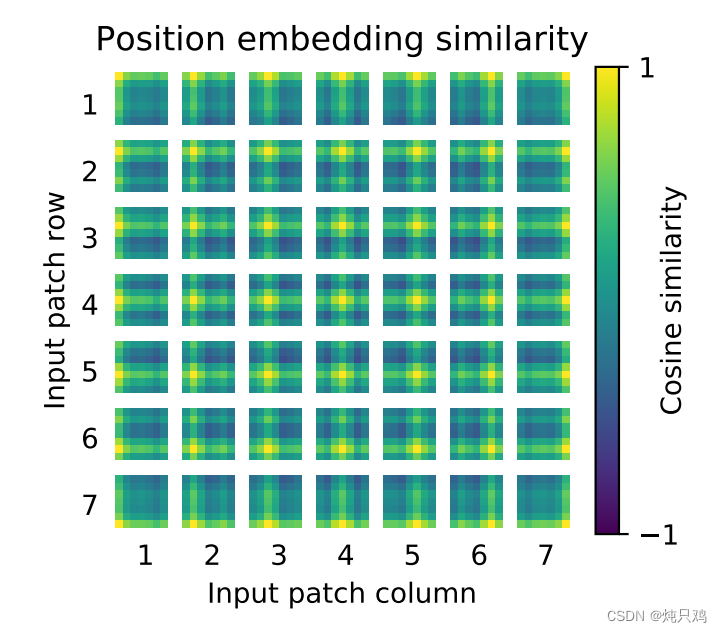
在输入Transformer Encoder之前注意需要加上[class]token以及Position Embedding。 在原论文中,作者说参考BERT,在刚刚得到的一堆tokens中插入一个专门用于分类的[class]token,这个[class]token是一个可训练的参数,数据格式和其他token一样都是一个向量,以ViT-B/16为例,就是一个长度为768的向量,与之前从图片中生成的tokens拼接在一起,Cat([1, 768], [196, 768]) -> [197, 768]。这里的Position Embedding采用的是一个可训练的参数(1D Pos. Emb.),是直接叠加在tokens上的(add),所以shape要一样。以ViT-B/16为例,刚刚拼接[class]token后shape是[197, 768],那么这里的Position Embedding的shape也是[197, 768]。
训练得到的位置编码他的每一个位置上与其他位置的余弦相似度图:
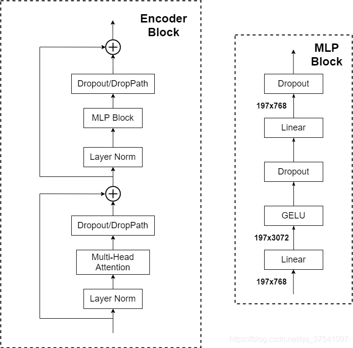
Transformer Encoder其实就是重复堆叠Encoder Block L次,下图是Encoder Block,主要由以下几部分组成:
- Layer Norm,这种Normalization方法主要是针对NLP领域提出的,这里是对每个token进行Norm处理。
- Multi-Head Attention。
- Dropout/DropPath,在原论文的代码中是直接使用的Dropout层,在但rwightman实现的代码中使用的是DropPath(stochastic depth),可能后者会更好一点。
- MLP Block,如图右侧所示,就是全连接+GELU激活函数+Dropout组成也非常简单,需要注意的是第一个全连接层会把输入节点个数翻4倍[197, 768] -> [197, 3072],第二个全连接层会还原回原节点个数[197, 3072] -> [197, 768]
MLP Head层结构
上面通过Transformer Encoder后输出的shape和输入的shape是保持不变的,以ViT-B/16为例,输入的是[197, 768]输出的还是[197, 768]。注意,在Transformer Encoder后其实还有一个Layer Norm没有画出来。这里只是需要分类的信息,所以只需要提取出[class]token生成的对应结果就行,即[197, 768]中抽取出[class]token对应的[1, 768]。接着通过MLP Head得到最终的分类结果。MLP Head原论文中说在训练ImageNet21K时是由Linear+tanh激活函数+Linear组成。但是迁移到ImageNet1K上或者自己的数据上时,只用一个Linear即可。
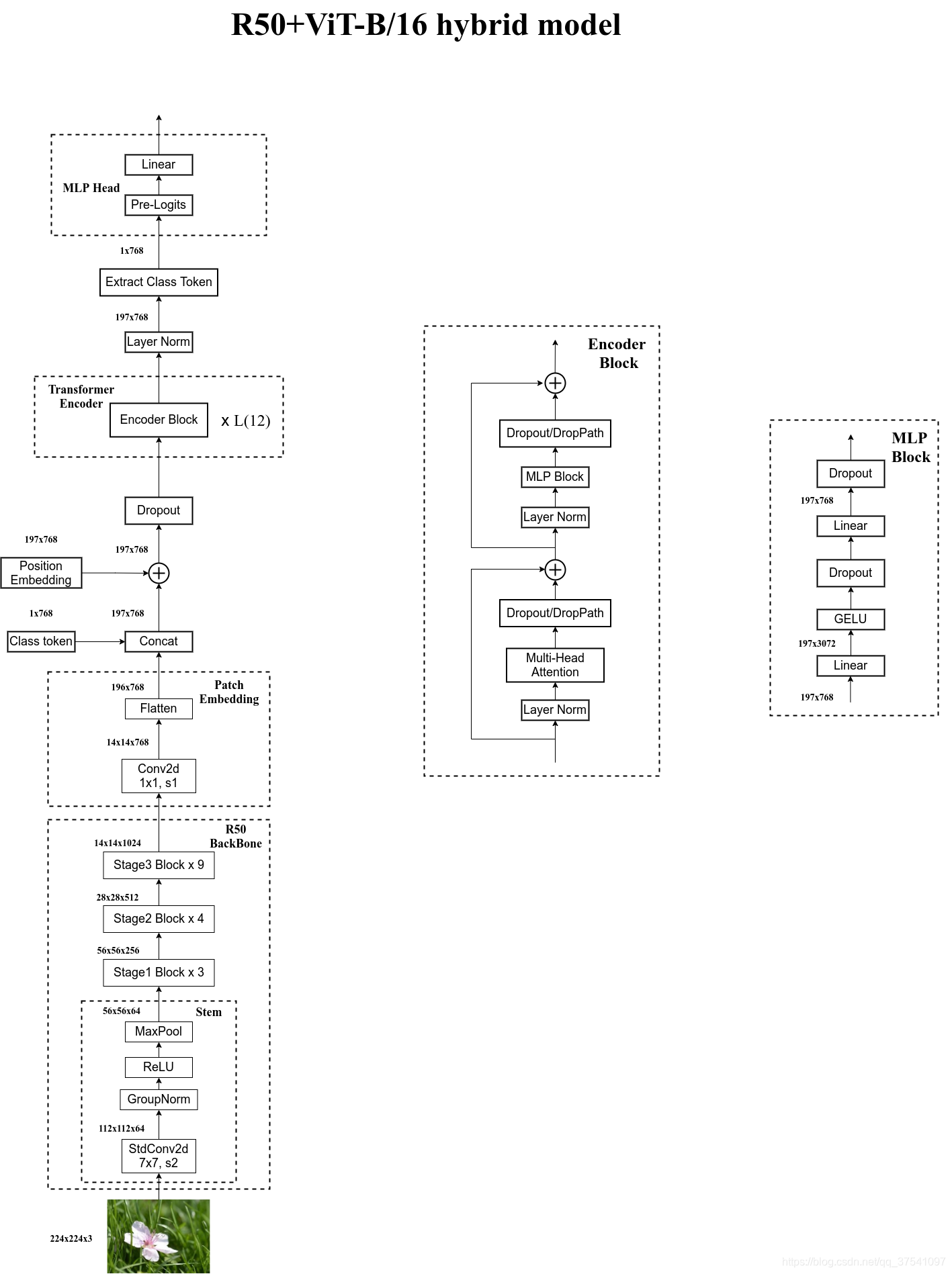
Hybrid模型
将传统CNN特征提取和Transformer进行结合。下图绘制的是以ResNet50作为特征提取器的混合模型,但这里的Resnet与之前讲的Resnet有些不同。首先这里的R50的卷积层采用的StdConv2d不是传统的Conv2d,然后将所有的BatchNorm层替换成GroupNorm层。在原Resnet50网络中,stage1重复堆叠3次,stage2重复堆叠4次,stage3重复堆叠6次,stage4重复堆叠3次,但在这里的R50中,把stage4中的3个Block移至stage3中,所以stage3中共重复堆叠9次。
通过R50 Backbone进行特征提取后,得到的特征矩阵shape是[14, 14, 1024],接着再输入Patch Embedding层,注意Patch Embedding中卷积层Conv2d的kernel_size和stride都变成了1,只是用来调整channel。后面的部分和前面ViT中讲的完全一样。
代码地址
deep-learning-for-image-processing/tensorflow_classification/vision_transformer at master · WZMIAOMIAO/deep-learning-for-image-processing · GitHubss
model
"""
refer to:
https://github.com/rwightman/pytorch-image-models/blob/master/timm/models/vision_transformer.py
"""
import tensorflow as tf
from tensorflow.keras import Model, layers, initializers
import numpy as np


class PatchEmbed(layers.Layer):
    """
    2D Image to Patch Embedding
    """
    def __init__(self, img_size=224, patch_size=16, embed_dim=768):
        super(PatchEmbed, self).__init__()
        self.embed_dim = embed_dim
        self.img_size = (img_size, img_size)
        self.grid_size = (img_size // patch_size, img_size // patch_size)
        self.num_patches = self.grid_size[0] * self.grid_size[1]

        self.proj = layers.Conv2D(filters=embed_dim, kernel_size=patch_size,
                                  strides=patch_size, padding='SAME',
                                  kernel_initializer=initializers.LecunNormal(),
                                  bias_initializer=initializers.Zeros())

    def call(self, inputs, **kwargs):
        B, H, W, C = inputs.shape
        assert H == self.img_size[0] and W == self.img_size[1], \
            f"Input image size ({H}*{W}) doesn't match model ({self.img_size[0]}*{self.img_size[1]})."  # 断言输入图像大小和固定大小一致
        x = self.proj(inputs)
        # [B, H, W, C] -> [B, H*W, C] 展平处理
        x = tf.reshape(x, [B, self.num_patches, self.embed_dim])
        return x


class ConcatClassTokenAddPosEmbed(layers.Layer):
    def __init__(self, embed_dim=768, num_patches=196, name=None):
        super(ConcatClassTokenAddPosEmbed, self).__init__(name=name)
        self.embed_dim = embed_dim
        self.num_patches = num_patches

    def build(self, input_shape):
        self.cls_token = self.add_weight(name="cls",
                                         shape=[1, 1, self.embed_dim],
                                         initializer=initializers.Zeros(),
                                         trainable=True,
                                         dtype=tf.float32)
        self.pos_embed = self.add_weight(name="pos_embed",
                                         shape=[1, self.num_patches + 1, self.embed_dim],
                                         initializer=initializers.RandomNormal(stddev=0.02),
                                         trainable=True,
                                         dtype=tf.float32)

    def call(self, inputs, **kwargs):
        batch_size, _, _ = inputs.shape

        # [1, 1, 768] -> [B, 1, 768]
        cls_token = tf.broadcast_to(self.cls_token, shape=[batch_size, 1, self.embed_dim])
        x = tf.concat([cls_token, inputs], axis=1)  # [B, 197, 768]
        x = x + self.pos_embed

        return x


class Attention(layers.Layer):
    k_ini = initializers.GlorotUniform()
    b_ini = initializers.Zeros()

    def __init__(self,
                 dim,
                 num_heads=8,
                 qkv_bias=False,
                 qk_scale=None,
                 attn_drop_ratio=0.,
                 proj_drop_ratio=0.,
                 name=None):
        super(Attention, self).__init__(name=name)
        self.num_heads = num_heads
        head_dim = dim // num_heads
        self.scale = qk_scale or head_dim ** -0.5
        self.qkv = layers.Dense(dim * 3, use_bias=qkv_bias, name="qkv",
                                kernel_initializer=self.k_ini, bias_initializer=self.b_ini)
        self.attn_drop = layers.Dropout(attn_drop_ratio)
        self.proj = layers.Dense(dim, name="out",
                                 kernel_initializer=self.k_ini, bias_initializer=self.b_ini)
        self.proj_drop = layers.Dropout(proj_drop_ratio)

    def call(self, inputs, training=None):
        # [batch_size, num_patches + 1, total_embed_dim]
        B, N, C = inputs.shape

        # qkv(): -> [batch_size, num_patches + 1, 3 * total_embed_dim]
        qkv = self.qkv(inputs)
        # reshape: -> [batch_size, num_patches + 1, 3, num_heads, embed_dim_per_head]
        qkv = tf.reshape(qkv, [B, N, 3, self.num_heads, C // self.num_heads])
        # transpose: -> [3, batch_size, num_heads, num_patches + 1, embed_dim_per_head]
        qkv = tf.transpose(qkv, [2, 0, 3, 1, 4])  # 调整位置
        # [batch_size, num_heads, num_patches + 1, embed_dim_per_head]
        q, k, v = qkv[0], qkv[1], qkv[2]  # 通过切片的方式分别取出qkv

        # transpose: -> [batch_size, num_heads, embed_dim_per_head, num_patches + 1]
        # multiply -> [batch_size, num_heads, num_patches + 1, num_patches + 1]
        attn = tf.matmul(a=q, b=k, transpose_b=True) * self.scale
        attn = tf.nn.softmax(attn, axis=-1)
        attn = self.attn_drop(attn, training=training)

        # multiply -> [batch_size, num_heads, num_patches + 1, embed_dim_per_head]
        x = tf.matmul(attn, v)
        # transpose: -> [batch_size, num_patches + 1, num_heads, embed_dim_per_head]
        x = tf.transpose(x, [0, 2, 1, 3])
        # reshape: -> [batch_size, num_patches + 1, total_embed_dim]
        x = tf.reshape(x, [B, N, C])

        x = self.proj(x)
        x = self.proj_drop(x, training=training)
        return x


class MLP(layers.Layer):
    """
    MLP as used in Vision Transformer, MLP-Mixer and related networks
    """

    k_ini = initializers.GlorotUniform()
    b_ini = initializers.RandomNormal(stddev=1e-6)

    def __init__(self, in_features, mlp_ratio=4.0, drop=0., name=None):
        super(MLP, self).__init__(name=name)
        self.fc1 = layers.Dense(int(in_features * mlp_ratio), name="Dense_0",
                                kernel_initializer=self.k_ini, bias_initializer=self.b_ini)
        self.act = layers.Activation("gelu")
        self.fc2 = layers.Dense(in_features, name="Dense_1",
                                kernel_initializer=self.k_ini, bias_initializer=self.b_ini)
        self.drop = layers.Dropout(drop)

    def call(self, inputs, training=None):
        x = self.fc1(inputs)
        x = self.act(x)
        x = self.drop(x, training=training)
        x = self.fc2(x)
        x = self.drop(x, training=training)
        return x


class Block(layers.Layer):
    def __init__(self,
                 dim,
                 num_heads=8,
                 qkv_bias=False,
                 qk_scale=None,
                 drop_ratio=0.,
                 attn_drop_ratio=0.,
                 drop_path_ratio=0.,
                 name=None):
        super(Block, self).__init__(name=name)
        self.norm1 = layers.LayerNormalization(epsilon=1e-6, name="LayerNorm_0")
        self.attn = Attention(dim, num_heads=num_heads,
                              qkv_bias=qkv_bias, qk_scale=qk_scale,
                              attn_drop_ratio=attn_drop_ratio, proj_drop_ratio=drop_ratio,
                              name="MultiHeadAttention")
        # NOTE: drop path for stochastic depth, we shall see if this is better than dropout here
        self.drop_path = layers.Dropout(rate=drop_path_ratio, noise_shape=(None, 1, 1)) if drop_path_ratio > 0. \
            else layers.Activation("linear")
        self.norm2 = layers.LayerNormalization(epsilon=1e-6, name="LayerNorm_1")
        self.mlp = MLP(dim, drop=drop_ratio, name="MlpBlock")

    def call(self, inputs, training=None):
        x = inputs + self.drop_path(self.attn(self.norm1(inputs)), training=training)
        x = x + self.drop_path(self.mlp(self.norm2(x)), training=training)
        return x


class VisionTransformer(Model):
    def __init__(self, img_size=224, patch_size=16, embed_dim=768,
                 depth=12, num_heads=12, qkv_bias=True, qk_scale=None,
                 drop_ratio=0., attn_drop_ratio=0., drop_path_ratio=0.,
                 representation_size=None, num_classes=1000, name="ViT-B/16"):
        super(VisionTransformer, self).__init__(name=name)
        self.num_classes = num_classes
        self.embed_dim = embed_dim
        self.depth = depth
        self.qkv_bias = qkv_bias

        self.patch_embed = PatchEmbed(img_size=img_size, patch_size=patch_size, embed_dim=embed_dim)
        num_patches = self.patch_embed.num_patches
        self.cls_token_pos_embed = ConcatClassTokenAddPosEmbed(embed_dim=embed_dim,
                                                               num_patches=num_patches,
                                                               name="cls_pos")

        self.pos_drop = layers.Dropout(drop_ratio)

        dpr = np.linspace(0., drop_path_ratio, depth)  # stochastic depth decay rule
        self.blocks = [Block(dim=embed_dim, num_heads=num_heads, qkv_bias=qkv_bias,
                             qk_scale=qk_scale, drop_ratio=drop_ratio, attn_drop_ratio=attn_drop_ratio,
                             drop_path_ratio=dpr[i], name="encoderblock_{}".format(i))
                       for i in range(depth)]

        self.norm = layers.LayerNormalization(epsilon=1e-6, name="encoder_norm")

        if representation_size:
            self.has_logits = True
            self.pre_logits = layers.Dense(representation_size, activation="tanh", name="pre_logits")
        else:
            self.has_logits = False
            self.pre_logits = layers.Activation("linear")

        self.head = layers.Dense(num_classes, name="head", kernel_initializer=initializers.Zeros())

    def call(self, inputs, training=None):
        # [B, H, W, C] -> [B, num_patches, embed_dim]
        x = self.patch_embed(inputs)  # [B, 196, 768]
        x = self.cls_token_pos_embed(x)  # [B, 176, 768]
        x = self.pos_drop(x, training=training)

        for block in self.blocks:
            x = block(x, training=training)

        x = self.norm(x)
        x = self.pre_logits(x[:, 0])
        x = self.head(x)

        return x


def vit_base_patch16_224_in21k(num_classes: int = 21843, has_logits: bool = True):
    """
    ViT-Base model (ViT-B/16) from original paper (https://arxiv.org/abs/2010.11929).
    ImageNet-21k weights @ 224x224, source https://github.com/google-research/vision_transformer.
    """
    model = VisionTransformer(img_size=224,
                              patch_size=16,
                              embed_dim=768,
                              depth=12,
                              num_heads=12,
                              representation_size=768 if has_logits else None,
                              num_classes=num_classes,
                              name="ViT-B_16")
    return model


def vit_base_patch32_224_in21k(num_classes: int = 21843, has_logits: bool = True):
    """
    ViT-Base model (ViT-B/32) from original paper (https://arxiv.org/abs/2010.11929).
    ImageNet-21k weights @ 224x224, source https://github.com/google-research/vision_transformer.
    """
    model = VisionTransformer(img_size=224,
                              patch_size=32,
                              embed_dim=768,
                              depth=12,
                              num_heads=12,
                              representation_size=768 if has_logits else None,
                              num_classes=num_classes,
                              name="ViT-B_32")
    return model


def vit_large_patch16_224_in21k(num_classes: int = 21843, has_logits: bool = True):
    """
    ViT-Large model (ViT-L/16) from original paper (https://arxiv.org/abs/2010.11929).
    ImageNet-21k weights @ 224x224, source https://github.com/google-research/vision_transformer.
    """
    model = VisionTransformer(img_size=224,
                              patch_size=16,
                              embed_dim=1024,
                              depth=24,
                              num_heads=16,
                              representation_size=1024 if has_logits else None,
                              num_classes=num_classes,
                              name="ViT-L_16")
    return model


def vit_large_patch32_224_in21k(num_classes: int = 21843, has_logits: bool = True):
    """
    ViT-Large model (ViT-L/32) from original paper (https://arxiv.org/abs/2010.11929).
    ImageNet-21k weights @ 224x224, source https://github.com/google-research/vision_transformer.
    """
    model = VisionTransformer(img_size=224,
                              patch_size=32,
                              embed_dim=1024,
                              depth=24,
                              num_heads=16,
                              representation_size=1024 if has_logits else None,
                              num_classes=num_classes,
                              name="ViT-L_32")
    return model


def vit_huge_patch14_224_in21k(num_classes: int = 21843, has_logits: bool = True):
    """
    ViT-Huge model (ViT-H/14) from original paper (https://arxiv.org/abs/2010.11929).
    ImageNet-21k weights @ 224x224, source https://github.com/google-research/vision_transformer.
    """
    model = VisionTransformer(img_size=224,
                              patch_size=14,
                              embed_dim=1280,
                              depth=32,
                              num_heads=16,
                              representation_size=1280 if has_logits else None,
                              num_classes=num_classes,
                              name="ViT-H_14")
    return model