为熟悉jupyter,找了一本书练习。
参考资料:《Python数据挖掘入门与实践》
数据集:
https://github.com/packtpublishing/learning-data-mining-with-python
第一行代码
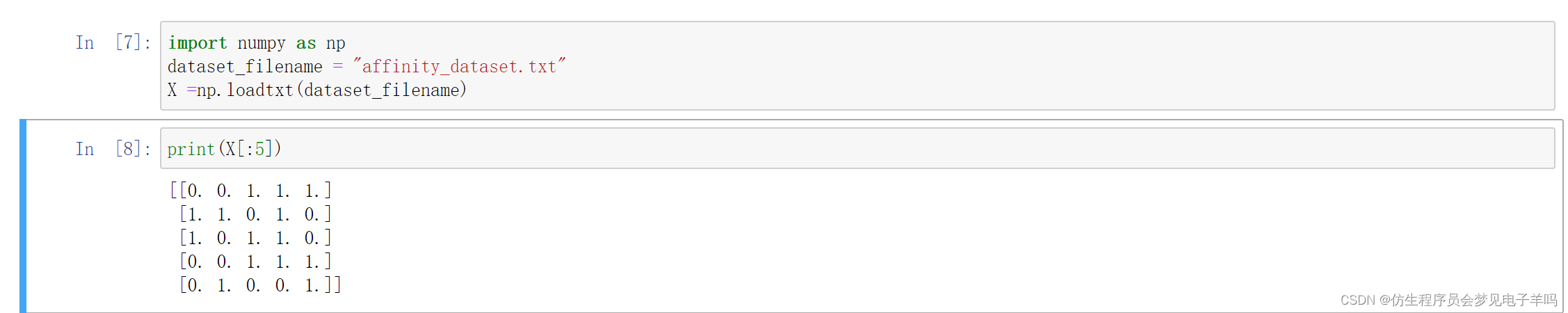
import numpy as np
dataset_filename = "affinity_dataset.txt"
X =np.loadtxt(dataset_filename)
print(X[:5])
[[0. 0. 1. 1. 1.]
[1. 1. 0. 1. 0.]
[1. 0. 1. 1. 0.]
[0. 0. 1. 1. 1.]
[0. 1. 0. 0. 1.]]
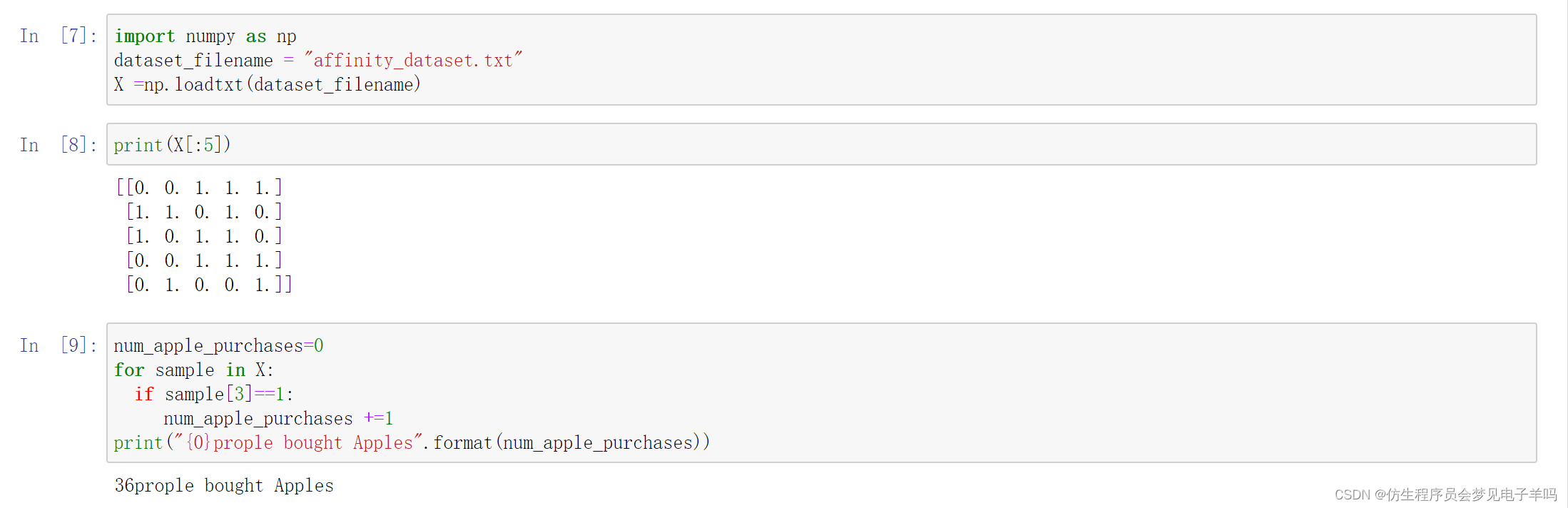
num_apple_purchases=0
for sample in X:
  if sample[3]==1:
     num_apple_purchases +=1
print("{0}prople bought Apples".format(num_apple_purchases))
分类
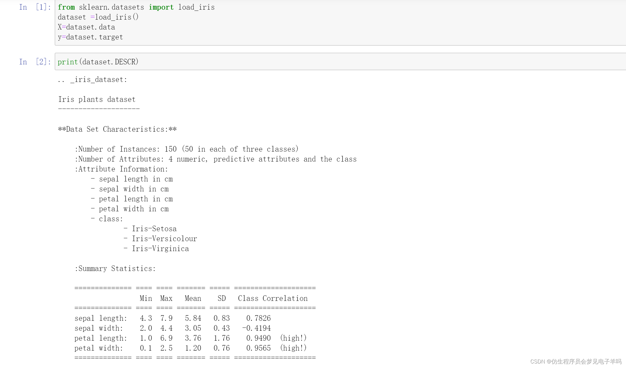
鸢尾花数据集
from sklearn.datasets import load_iris
dataset =load_iris()
X=dataset.data
y=dataset.target
print(dataset.DESCR)
把连续值转变为类别型,这个过程叫做离散化。
最简单的离散化方法,莫过于确定一个阈值,将低于该阈值的特征值置为0,高于阈值的置为1.
我们把某项特征的阈值设定为该特征所有特征值的均值。
每个特征的均值计算方法如下:
attribute_means =X.mean(axis=0)
我们得到了一个长度为4的数组,这是特征的数量。
数组的第一项是第一个特征的均值,以此类推。
接下来,用该方法将数据集打散,把连续的特征值转换为类别型。
X_d=np.array(X >= attribute_means,dtype='int')
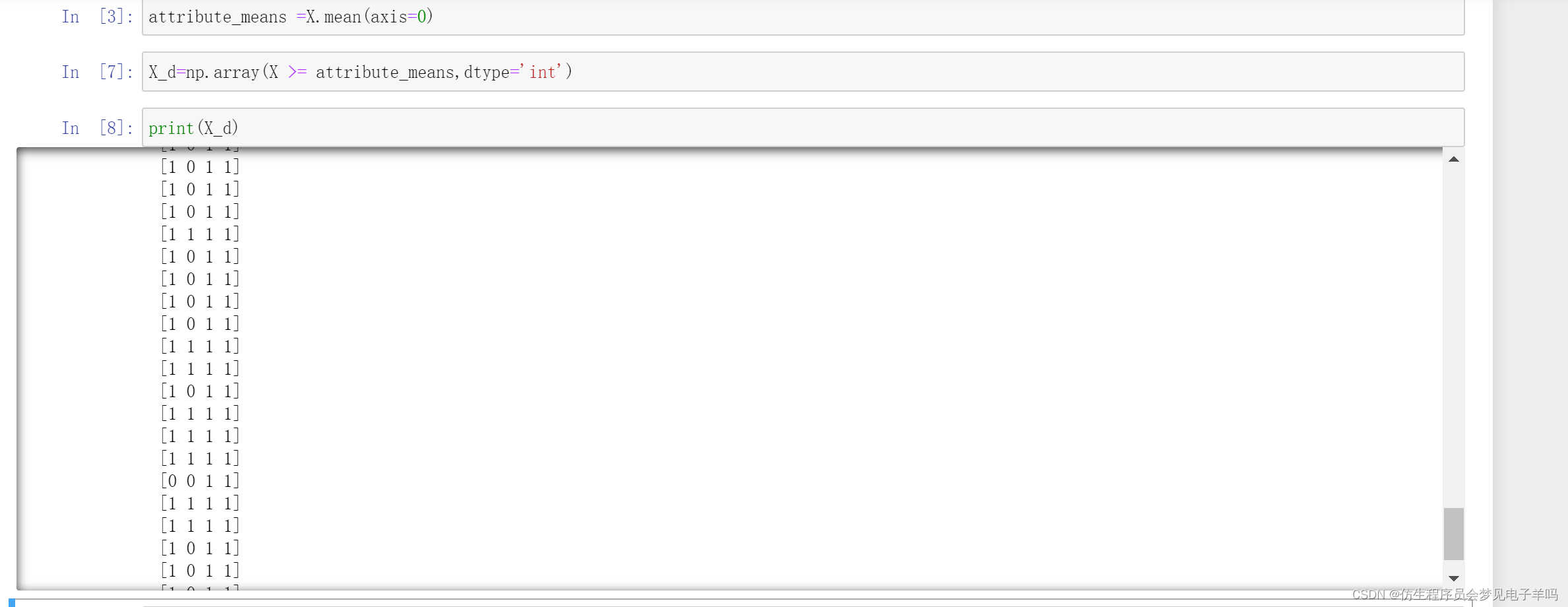
后面的训练和测试,都将用到新得到的X_d数据集(打散后的数组X),而不使用原来的数据集(X)
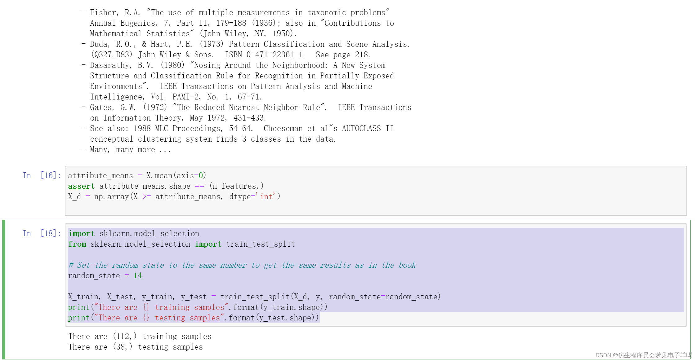
attribute_means = X.mean(axis=0)
assert attribute_means.shape == (n_features,)
X_d = np.array(X >= attribute_means, dtype='int')
import sklearn.model_selection
from sklearn.model_selection import train_test_split

# Set the random state to the same number to get the same results as in the book
random_state = 14

X_train, X_test, y_train, y_test = train_test_split(X_d, y, random_state=random_state)
print("There are {} training samples".format(y_train.shape))
print("There are {} testing samples".format(y_test.shape))
There are (112,) training samples
There are (38,) testing samples
from collections import defaultdict
from operator import itemgetter


def train(X, y_true, feature):
    """Computes the predictors and error for a given feature using the OneR algorithm

    Parameters
    ----------
    X: array [n_samples, n_features]
        The two dimensional array that holds the dataset. Each row is a sample, each column
        is a feature.

    y_true: array [n_samples,]
        The one dimensional array that holds the class values. Corresponds to X, such that
        y_true[i] is the class value for sample X[i].

    feature: int
        An integer corresponding to the index of the variable we wish to test.
        0 <= variable < n_features

    Returns
    -------
    predictors: dictionary of tuples: (value, prediction)
        For each item in the array, if the variable has a given value, make the given prediction.

    error: float
        The ratio of training data that this rule incorrectly predicts.
    """
    # Check that variable is a valid number
    n_samples, n_features = X.shape
    assert 0 <= feature < n_features
    # Get all of the unique values that this variable has
    values = set(X[:,feature])
    # Stores the predictors array that is returned
    predictors = dict()
    errors = []
    for current_value in values:
        most_frequent_class, error = train_feature_value(X, y_true, feature, current_value)
        predictors[current_value] = most_frequent_class
        errors.append(error)
    # Compute the total error of using this feature to classify on
    total_error = sum(errors)
    return predictors, total_error

# Compute what our predictors say each sample is based on its value
#y_predicted = np.array([predictors[sample[feature]] for sample in X])


def train_feature_value(X, y_true, feature, value):
    # Create a simple dictionary to count how frequency they give certain predictions
    class_counts = defaultdict(int)
    # Iterate through each sample and count the frequency of each class/value pair
    for sample, y in zip(X, y_true):
        if sample[feature] == value:
            class_counts[y] += 1
    # Now get the best one by sorting (highest first) and choosing the first item
    sorted_class_counts = sorted(class_counts.items(), key=itemgetter(1), reverse=True)
    most_frequent_class = sorted_class_counts[0][0]
    # The error is the number of samples that do not classify as the most frequent class
    # *and* have the feature value.
    n_samples = X.shape[1]
    error = sum([class_count for class_value, class_count in class_counts.items()
                 if class_value != most_frequent_class])
    return most_frequent_class, error
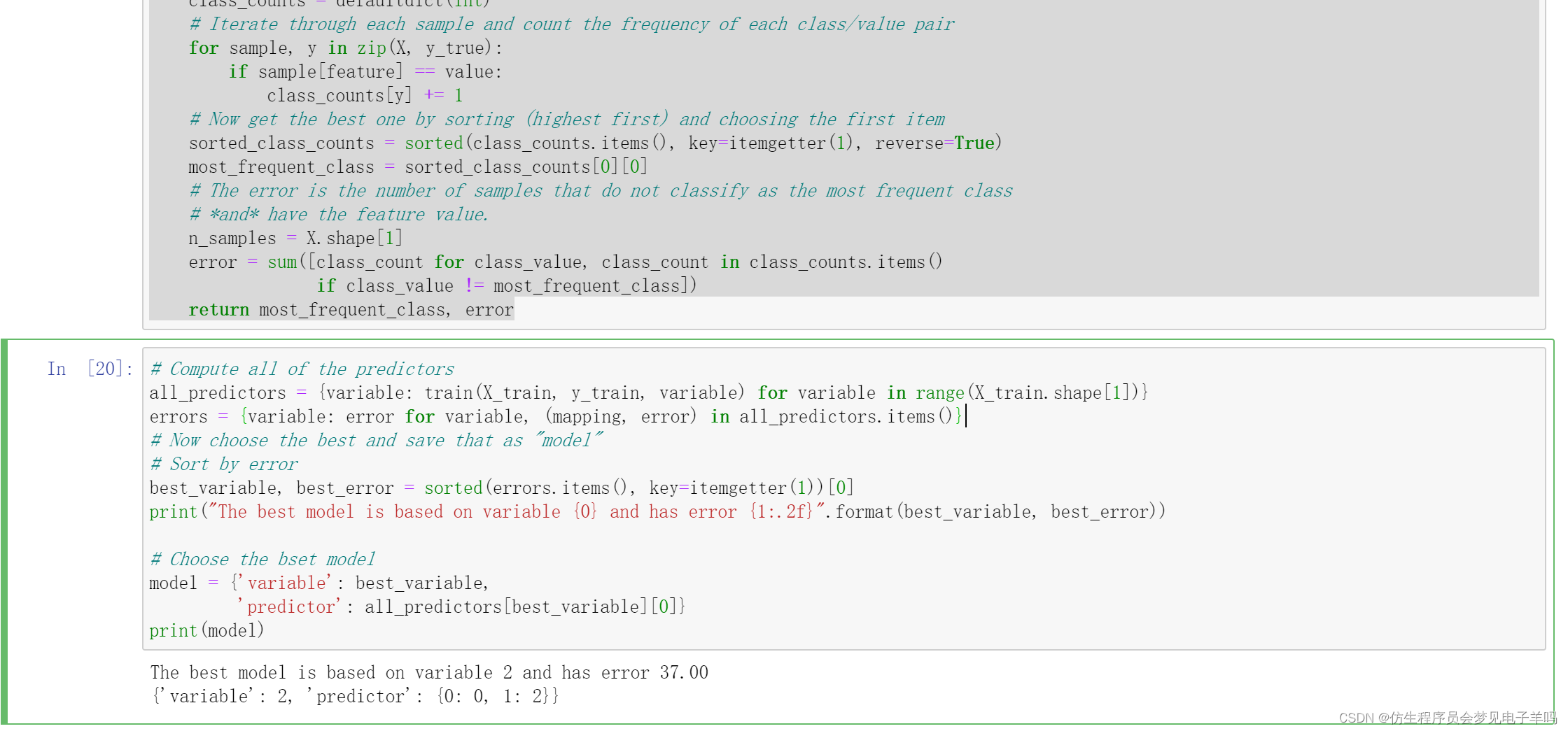
# Compute all of the predictors
all_predictors = {variable: train(X_train, y_train, variable) for variable in range(X_train.shape[1])}
errors = {variable: error for variable, (mapping, error) in all_predictors.items()}
# Now choose the best and save that as "model"
# Sort by error
best_variable, best_error = sorted(errors.items(), key=itemgetter(1))[0]
print("The best model is based on variable {0} and has error {1:.2f}".format(best_variable, best_error))

# Choose the bset model
model = {'variable': best_variable,
         'predictor': all_predictors[best_variable][0]}
print(model)
The best model is based on variable 2 and has error 37.00
{‘variable’: 2, ‘predictor’: {0: 0, 1: 2}}
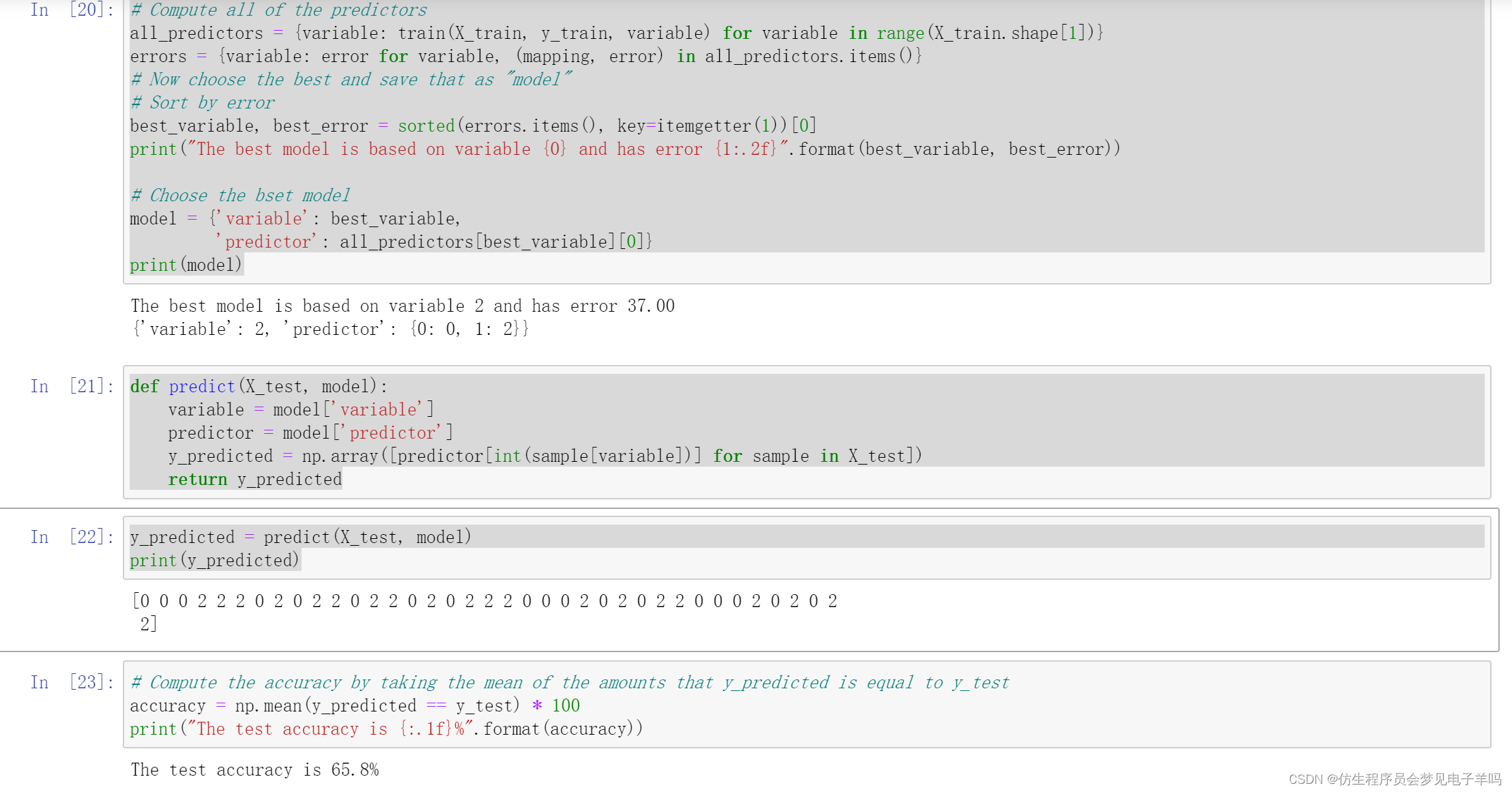
def predict(X_test, model):
    variable = model['variable']
    predictor = model['predictor']
    y_predicted = np.array([predictor[int(sample[variable])] for sample in X_test])
    return y_predicted
我们经常需要一次对多条数据进行预测,因此用代码实现这个函数,通过遍历数据集中的每条数据来完成预测。
y_predicted = predict(X_test, model)
print(y_predicted)
[0 0 0 2 2 2 0 2 0 2 2 0 2 2 0 2 0 2 2 2 0 0 0 2 0 2 0 2 2 0 0 0 2 0 2 0 2
2]
比较预测结果和实际类别,就能得到正确率是多少。
# Compute the accuracy by taking the mean of the amounts that y_predicted is equal to y_test
accuracy = np.mean(y_predicted == y_test) * 100
print("The test accuracy is {:.1f}%".format(accuracy))
The test accuracy is 65.8%
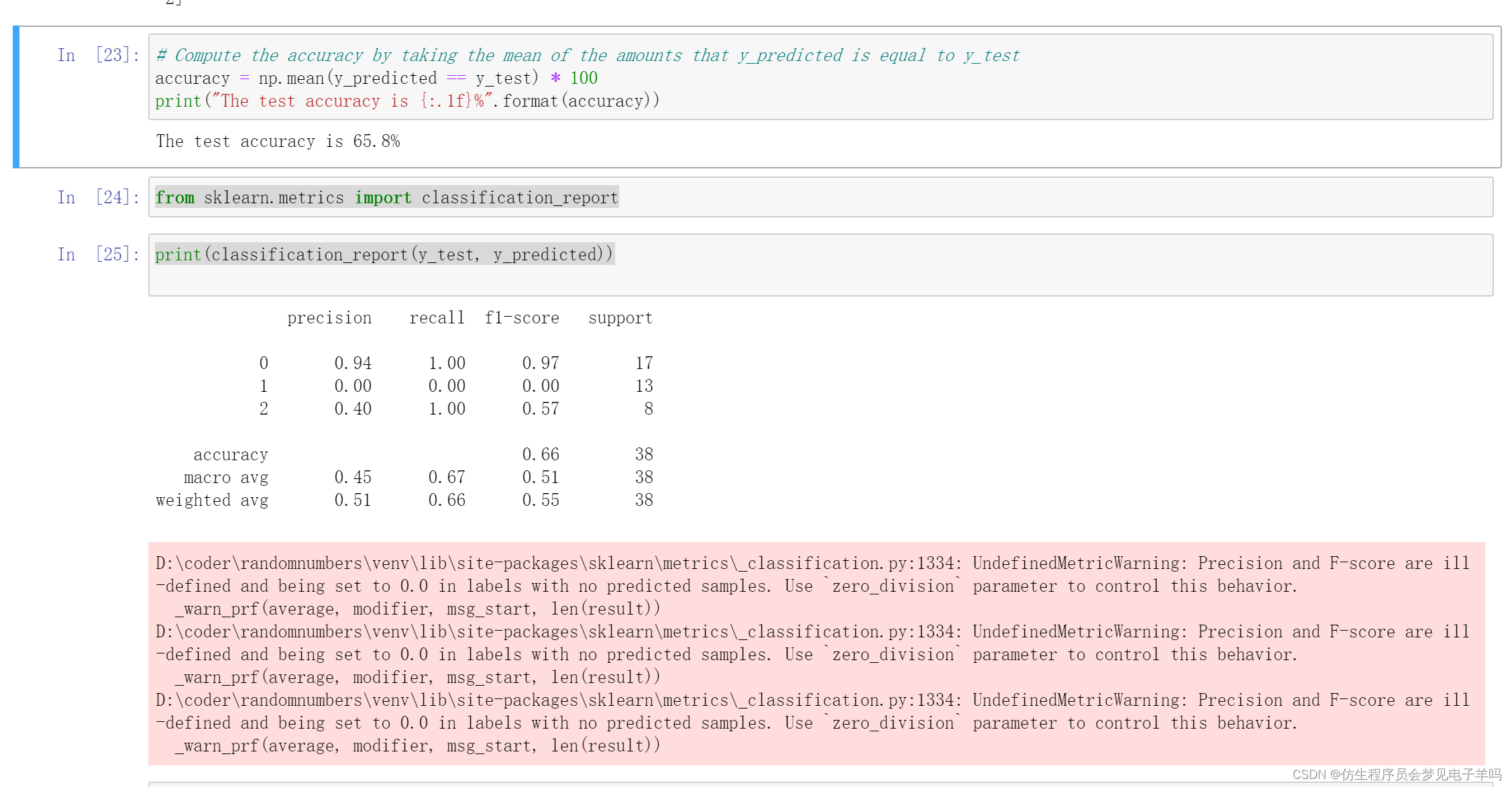
from sklearn.metrics import classification_report
print(classification_report(y_test, y_predicted))
近邻
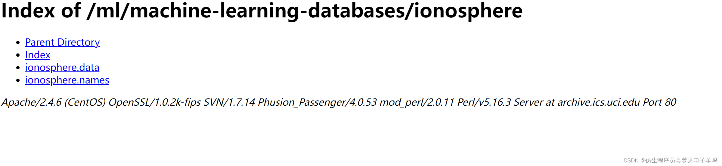
主目录位置
数据集:
http://archive.ics.uci.edu/ml/datasets/Ionosphere

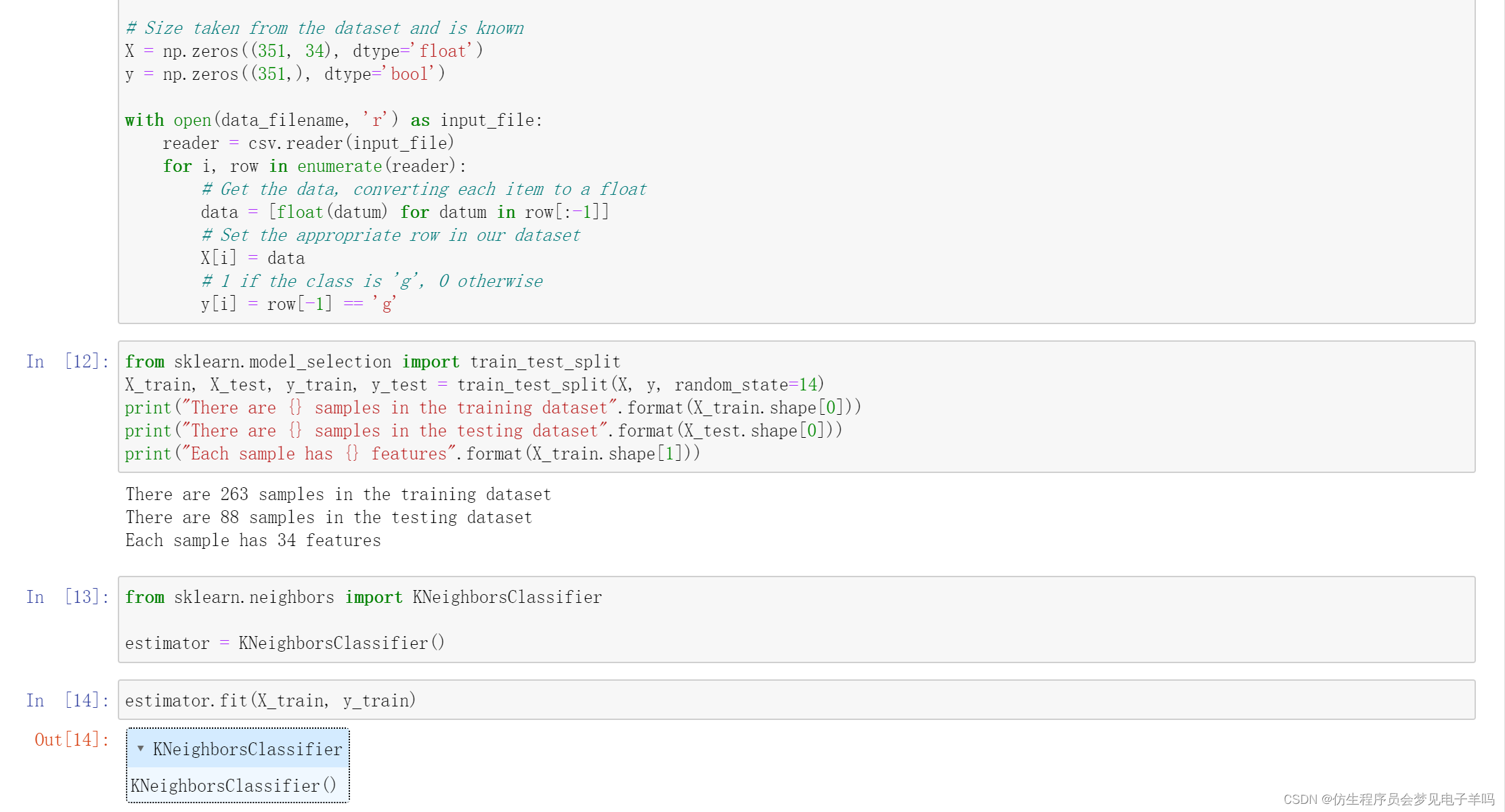
# Change this to the location of your dataset
data_folder = os.path.join(home_folder, "Data", "Ionosphere")
data_filename = os.path.join(data_folder, "ionosphere.data")
print(data_filename)
C:\Users\83854\Data\Ionosphere\ionosphere.data
import csv
import numpy as np

# Size taken from the dataset and is known
X = np.zeros((351, 34), dtype='float')
y = np.zeros((351,), dtype='bool')

with open(data_filename, 'r') as input_file:
    reader = csv.reader(input_file)
    for i, row in enumerate(reader):
        # Get the data, converting each item to a float
        data = [float(datum) for datum in row[:-1]]
        # Set the appropriate row in our dataset
        X[i] = data
        # 1 if the class is 'g', 0 otherwise
        y[i] = row[-1] == 'g'
from sklearn.model_selection import train_test_split
X_train, X_test, y_train, y_test = train_test_split(X, y, random_state=14)
print("There are {} samples in the training dataset".format(X_train.shape[0]))
print("There are {} samples in the testing dataset".format(X_test.shape[0]))
print("Each sample has {} features".format(X_train.shape[1]))
There are 263 samples in the training dataset
There are 88 samples in the testing dataset
Each sample has 34 features
from sklearn.neighbors import KNeighborsClassifier

estimator = KNeighborsClassifier()
estimator.fit(X_train, y_train)
y_predicted = estimator.predict(X_test)
accuracy = np.mean(y_test == y_predicted) * 100
print("The accuracy is {0:.1f}%".format(accuracy))
The accuracy is 86.4%
from sklearn.model_selection import cross_val_score
scores = cross_val_score(estimator, X, y, scoring='accuracy')
average_accuracy = np.mean(scores) * 100
print("The average accuracy is {0:.1f}%".format(average_accuracy))
The average accuracy is 82.6%
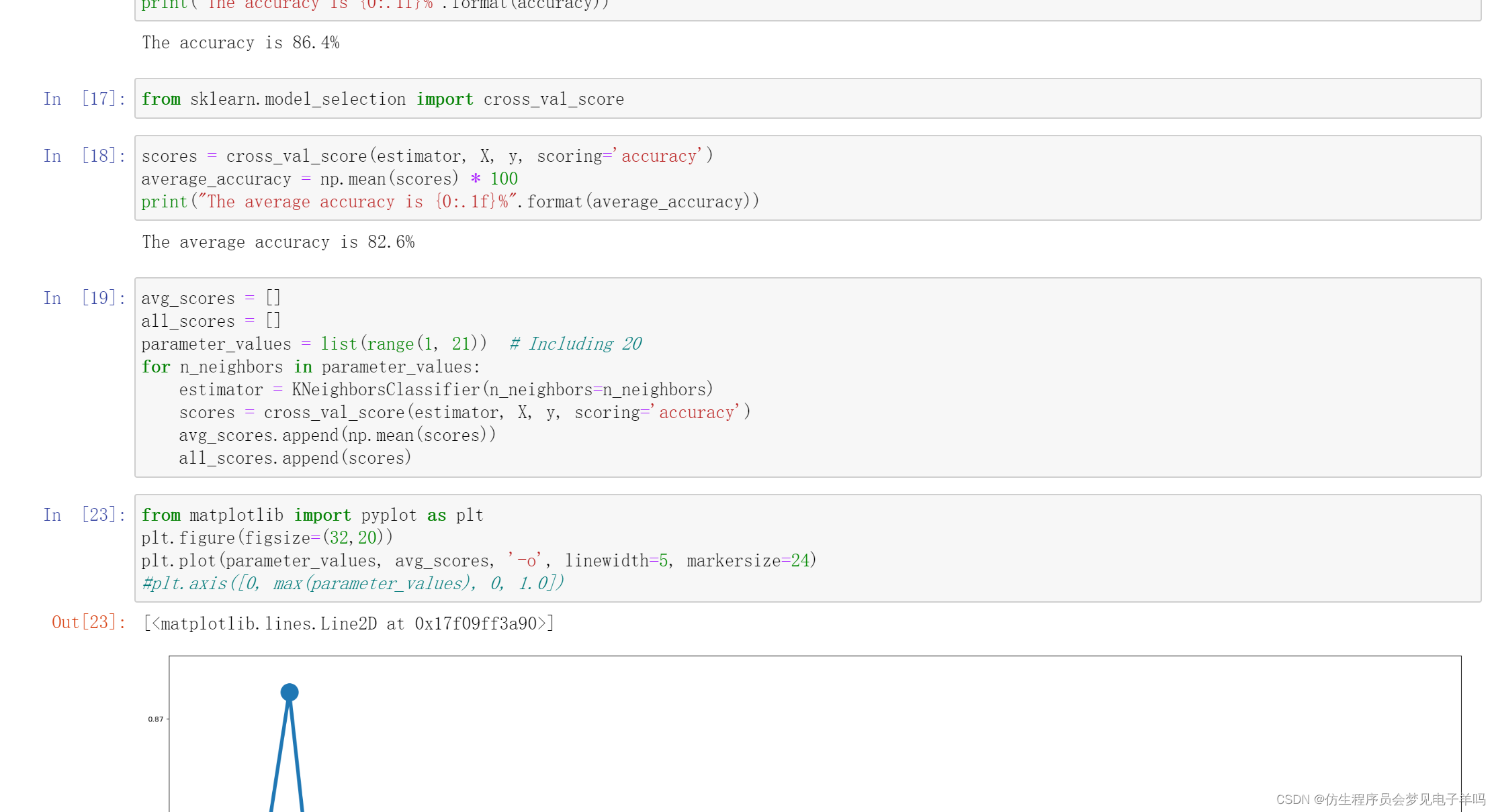
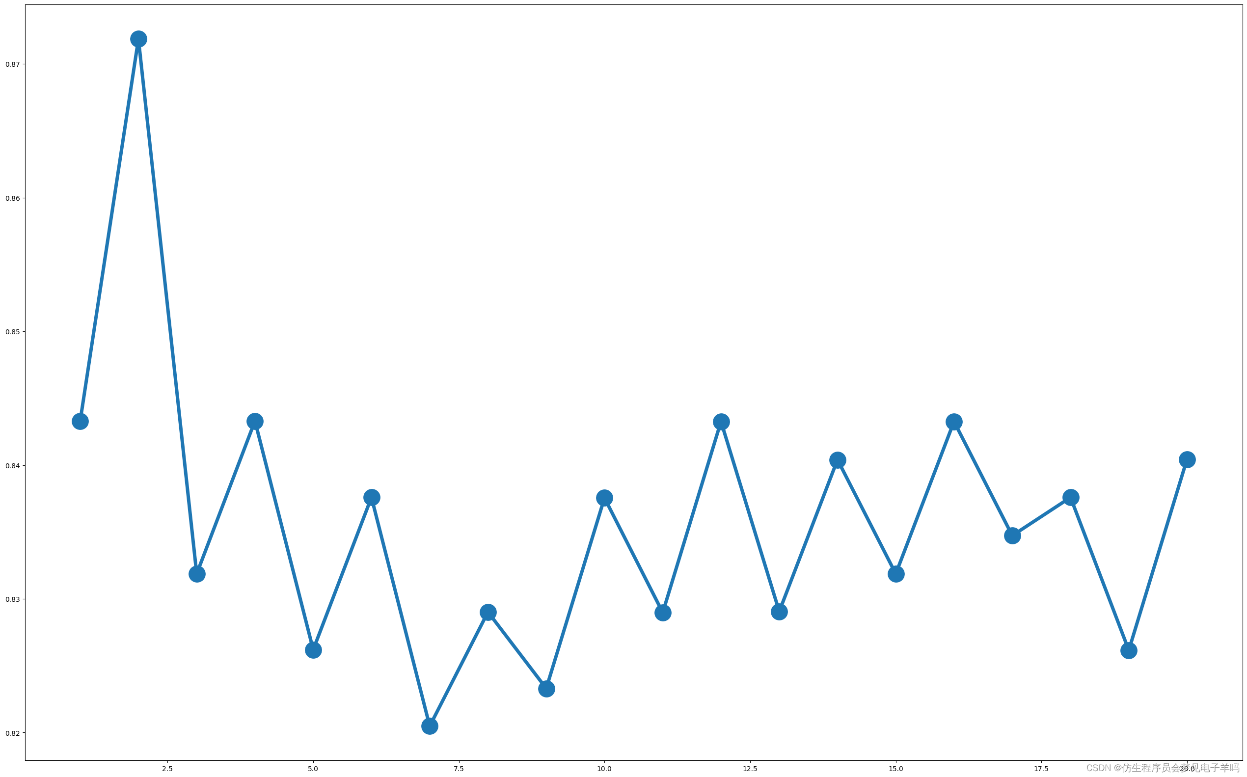
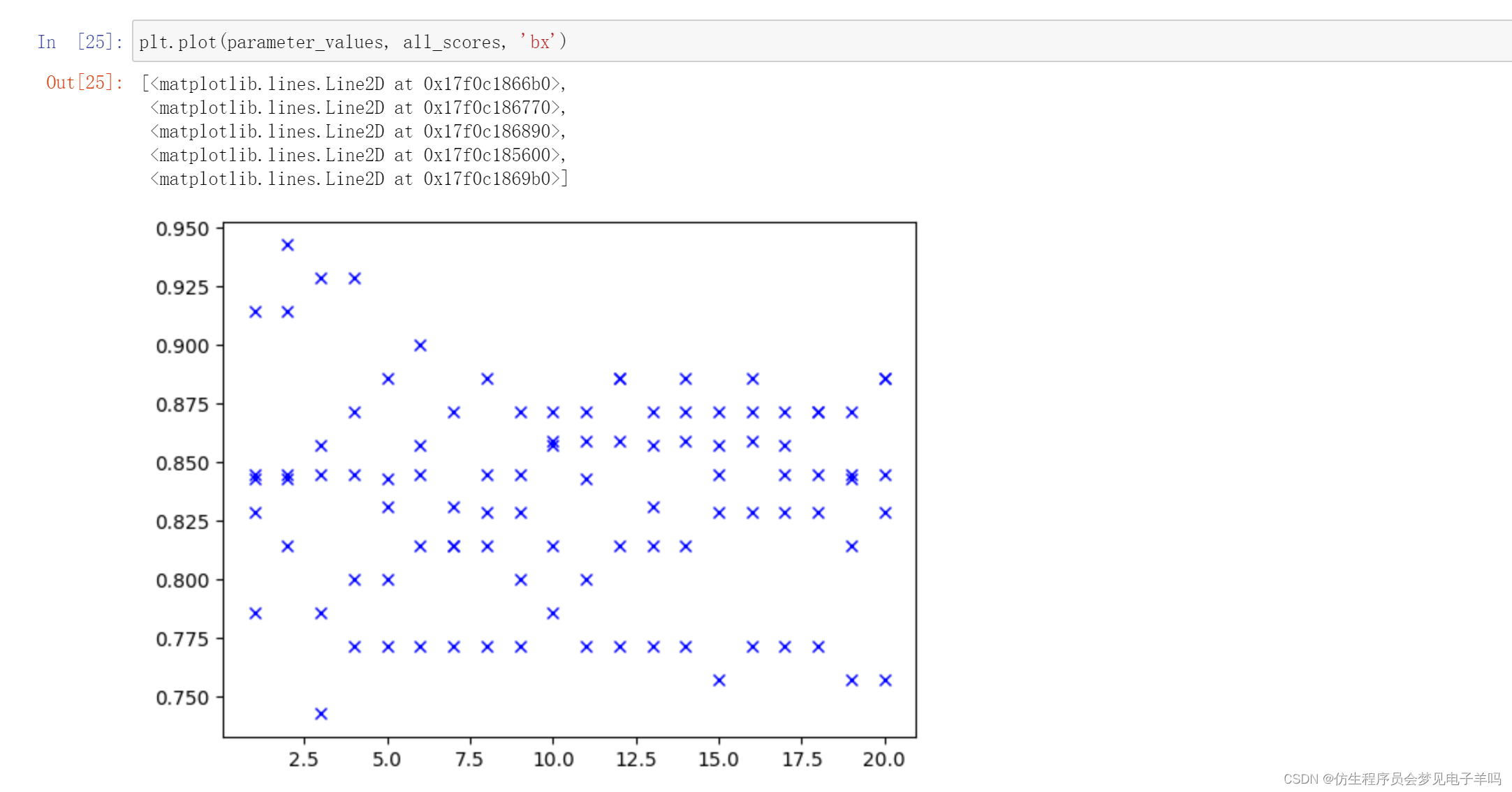
avg_scores = []
all_scores = []
parameter_values = list(range(1, 21))  # Including 20
for n_neighbors in parameter_values:
    estimator = KNeighborsClassifier(n_neighbors=n_neighbors)
    scores = cross_val_score(estimator, X, y, scoring='accuracy')
    avg_scores.append(np.mean(scores))
    all_scores.append(scores)
from matplotlib import pyplot as plt
plt.figure(figsize=(32,20))
plt.plot(parameter_values, avg_scores, '-o', linewidth=5, markersize=24)
#plt.axis([0, max(parameter_values), 0, 1.0])
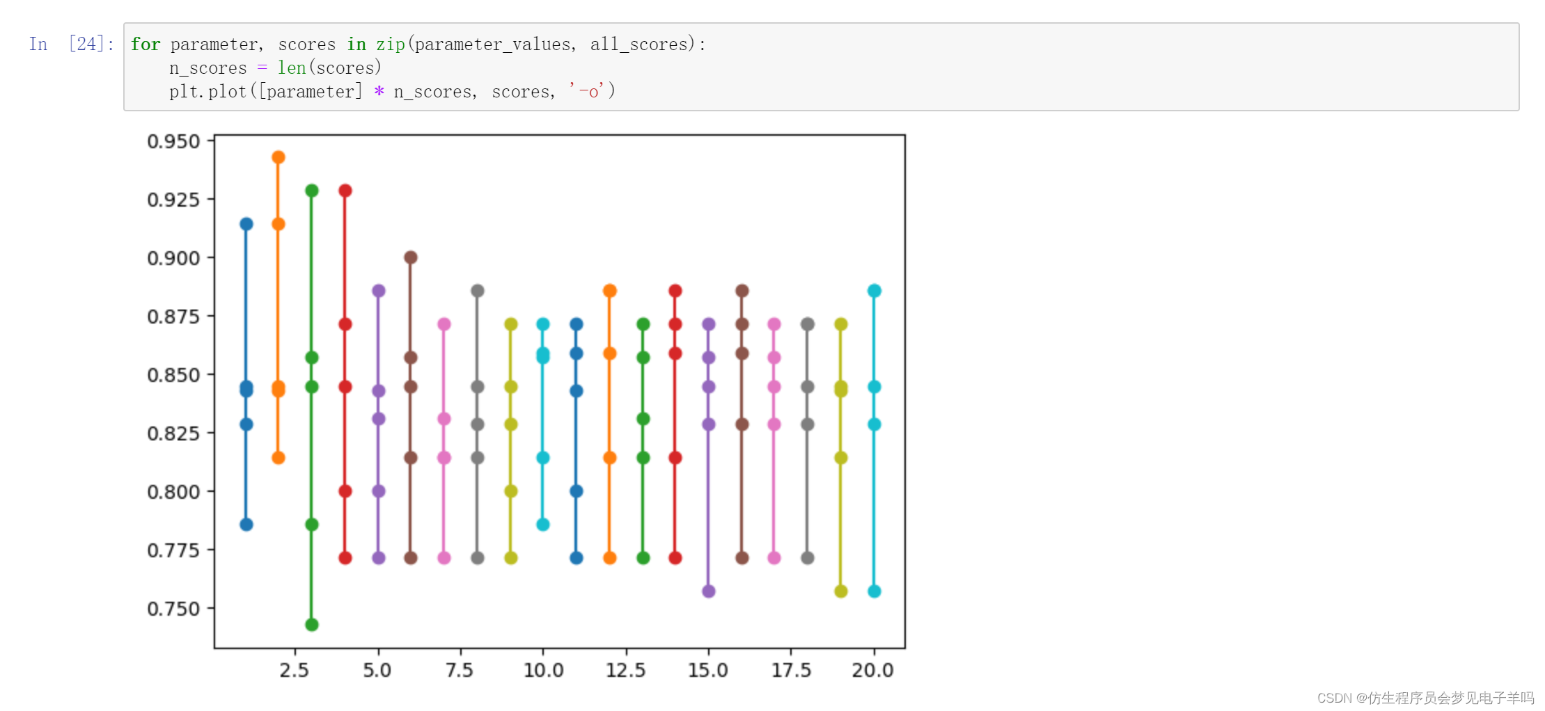
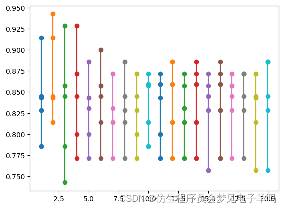
for parameter, scores in zip(parameter_values, all_scores):
    n_scores = len(scores)
    plt.plot([parameter] * n_scores, scores, '-o')
plt.plot(parameter_values, all_scores, 'bx')
[<matplotlib.lines.Line2D at 0x17f0c1866b0>,
<matplotlib.lines.Line2D at 0x17f0c186770>,
<matplotlib.lines.Line2D at 0x17f0c186890>,
<matplotlib.lines.Line2D at 0x17f0c185600>,
<matplotlib.lines.Line2D at 0x17f0c1869b0>]
电影推荐
数据集:
https://grouplens.org/datasets/movielens/
import os
import pandas as pd
#data_folder =os.path.join(os.path.expanduser("~"),"shujvji","ml-100k")
#ratings_filename=os.path.join(data_folder,"u.data")
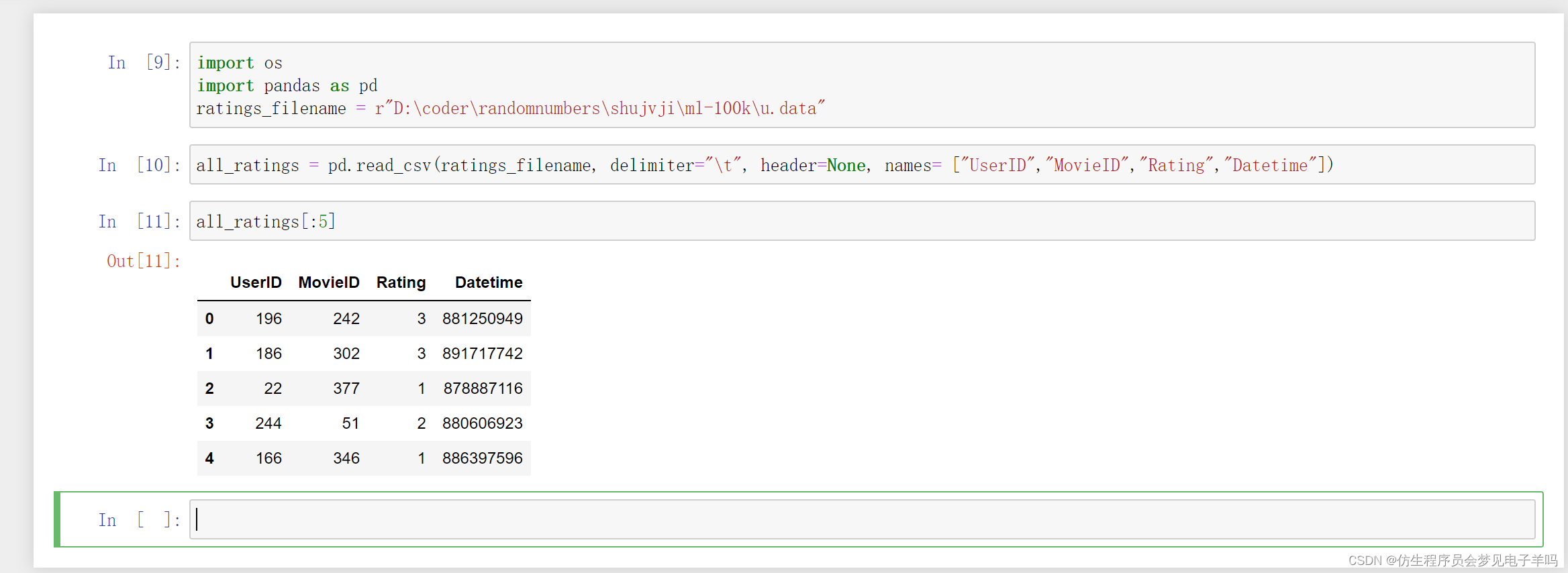
ratings_filename = r"D:\coder\randomnumbers\shujvji\ml-100k\u.data"
该数据集非常规整,但有几点与pandas.read_csv方法的默认设置有出入,所以要调整参数设置。
第一个问题是数据集每行的几个数据之间用制表符而不是逗号分隔。
其次,没有表头,这表示数据集的第一行就是数据部分,我们需要手动为各列添加名称。
all_ratings=pd.read_csv(ratings_filename,delimiter="\t",header=None,names=["UserID","MovieID","Rating","Datetime"])
运行下面代码,看一下前五条记录:
all_ratings[:5]
UserID MovieID Rating Datetime
0 196 242 3 881250949
1 186 302 3 891717742
2 22 377 1 878887116
3 244 51 2 880606923
4 166 346 1 886397596
完整代码
下面是完整代码:
import os
data_folder = os.path.join(os.path.expanduser("~"), "Data", "ml-100k")
ratings_filename = os.path.join(data_folder, "u.data")
import pandas as pd
all_ratings = pd.read_csv(ratings_filename, delimiter="\t", header=None, names = ["UserID", "MovieID", "Rating", "Datetime"])
all_ratings["Datetime"] = pd.to_datetime(all_ratings['Datetime'],unit='s')
all_ratings[:5]
|
UserID |
MovieID |
Rating |
Datetime |
| 0 |
196 |
242 |
3 |
1997-12-04 15:55:49 |
| 1 |
186 |
302 |
3 |
1998-04-04 19:22:22 |
| 2 |
22 |
377 |
1 |
1997-11-07 07:18:36 |
| 3 |
244 |
51 |
2 |
1997-11-27 05:02:03 |
| 4 |
166 |
346 |
1 |
1998-02-02 05:33:16 |
all_ratings[all_ratings["UserID"] == 675].sort_values("MovieID")
|
UserID |
MovieID |
Rating |
Datetime |
| 81098 |
675 |
86 |
4 |
1998-03-10 00:26:14 |
| 90696 |
675 |
223 |
1 |
1998-03-10 00:35:51 |
| 92650 |
675 |
235 |
1 |
1998-03-10 00:35:51 |
| 95459 |
675 |
242 |
4 |
1998-03-10 00:08:42 |
| 82845 |
675 |
244 |
3 |
1998-03-10 00:29:35 |
| 53293 |
675 |
258 |
3 |
1998-03-10 00:11:19 |
| 97286 |
675 |
269 |
5 |
1998-03-10 00:08:07 |
| 93720 |
675 |
272 |
3 |
1998-03-10 00:07:11 |
| 73389 |
675 |
286 |
4 |
1998-03-10 00:07:11 |
| 77524 |
675 |
303 |
5 |
1998-03-10 00:08:42 |
| 47367 |
675 |
305 |
4 |
1998-03-10 00:09:08 |
| 44300 |
675 |
306 |
5 |
1998-03-10 00:08:07 |
| 53730 |
675 |
311 |
3 |
1998-03-10 00:10:47 |
| 54284 |
675 |
312 |
2 |
1998-03-10 00:10:24 |
| 63291 |
675 |
318 |
5 |
1998-03-10 00:21:13 |
| 87082 |
675 |
321 |
2 |
1998-03-10 00:11:48 |
| 56108 |
675 |
344 |
4 |
1998-03-10 00:12:34 |
| 53046 |
675 |
347 |
4 |
1998-03-10 00:07:11 |
| 94617 |
675 |
427 |
5 |
1998-03-10 00:28:11 |
| 69915 |
675 |
463 |
5 |
1998-03-10 00:16:43 |
| 46744 |
675 |
509 |
5 |
1998-03-10 00:24:25 |
| 46598 |
675 |
531 |
5 |
1998-03-10 00:18:28 |
| 52962 |
675 |
650 |
5 |
1998-03-10 00:32:51 |
| 94029 |
675 |
750 |
4 |
1998-03-10 00:08:07 |
| 53223 |
675 |
874 |
4 |
1998-03-10 00:11:19 |
| 62277 |
675 |
891 |
2 |
1998-03-10 00:12:59 |
| 77274 |
675 |
896 |
5 |
1998-03-10 00:09:35 |
| 66194 |
675 |
900 |
4 |
1998-03-10 00:10:24 |
| 54994 |
675 |
937 |
1 |
1998-03-10 00:35:51 |
| 61742 |
675 |
1007 |
4 |
1998-03-10 00:25:22 |
| 49225 |
675 |
1101 |
4 |
1998-03-10 00:33:49 |
| 50692 |
675 |
1255 |
1 |
1998-03-10 00:35:51 |
| 74202 |
675 |
1628 |
5 |
1998-03-10 00:30:37 |
| 47866 |
675 |
1653 |
5 |
1998-03-10 00:31:53 |
all_ratings["Favorable"] = all_ratings["Rating"] > 3
all_ratings[10:15]
|
UserID |
MovieID |
Rating |
Datetime |
Favorable |
| 10 |
62 |
257 |
2 |
1997-11-12 22:07:14 |
False |
| 11 |
286 |
1014 |
5 |
1997-11-17 15:38:45 |
True |
| 12 |
200 |
222 |
5 |
1997-10-05 09:05:40 |
True |
| 13 |
210 |
40 |
3 |
1998-03-27 21:59:54 |
False |
| 14 |
224 |
29 |
3 |
1998-02-21 23:40:57 |
False |
all_ratings[all_ratings["UserID"] == 1][:5]
|
UserID |
MovieID |
Rating |
Datetime |
Favorable |
| 202 |
1 |
61 |
4 |
1997-11-03 07:33:40 |
True |
| 305 |
1 |
189 |
3 |
1998-03-01 06:15:28 |
False |
| 333 |
1 |
33 |
4 |
1997-11-03 07:38:19 |
True |
| 334 |
1 |
160 |
4 |
1997-09-24 03:42:27 |
True |
| 478 |
1 |
20 |
4 |
1998-02-14 04:51:23 |
True |
ratings = all_ratings[all_ratings['UserID'].isin(range(200))] # & ratings["UserID"].isin(range(100))]
favorable_ratings = ratings[ratings["Favorable"]]
favorable_ratings[:5]
|
UserID |
MovieID |
Rating |
Datetime |
Favorable |
| 16 |
122 |
387 |
5 |
1997-11-11 17:47:39 |
True |
| 20 |
119 |
392 |
4 |
1998-01-30 16:13:34 |
True |
| 21 |
167 |
486 |
4 |
1998-04-16 14:54:12 |
True |
| 26 |
38 |
95 |
5 |
1998-04-13 01:14:54 |
True |
| 28 |
63 |
277 |
4 |
1997-10-01 23:10:01 |
True |
favorable_reviews_by_users = dict((k, frozenset(v.values)) for k, v in favorable_ratings.groupby("UserID")["MovieID"])
len(favorable_reviews_by_users)
199
num_favorable_by_movie = ratings[["MovieID", "Favorable"]].groupby("MovieID").sum()
num_favorable_by_movie.sort_values("Favorable", ascending=False)[:5]
|
Favorable |
| MovieID |
|
| 50 |
100 |
| 100 |
89 |
| 258 |
83 |
| 181 |
79 |
| 174 |
74 |
from collections import defaultdict

def find_frequent_itemsets(favorable_reviews_by_users, k_1_itemsets, min_support):
    counts = defaultdict(int)
    for user, reviews in favorable_reviews_by_users.items():
        for itemset in k_1_itemsets:
            if itemset.issubset(reviews):
                for other_reviewed_movie in reviews - itemset:
                    current_superset = itemset | frozenset((other_reviewed_movie,))
                    counts[current_superset] += 1
    return dict([(itemset, frequency) for itemset, frequency in counts.items() if frequency >= min_support])
import sys
frequent_itemsets = {}  # itemsets are sorted by length
min_support = 50

# k=1 candidates are the isbns with more than min_support favourable reviews
frequent_itemsets[1] = dict((frozenset((movie_id,)), row["Favorable"])
                                for movie_id, row in num_favorable_by_movie.iterrows()
                                if row["Favorable"] > min_support)

print("There are {} movies with more than {} favorable reviews".format(len(frequent_itemsets[1]), min_support))
sys.stdout.flush()
for k in range(2, 20):
    # Generate candidates of length k, using the frequent itemsets of length k-1
    # Only store the frequent itemsets
    cur_frequent_itemsets = find_frequent_itemsets(favorable_reviews_by_users, frequent_itemsets[k-1],
                                                   min_support)
    if len(cur_frequent_itemsets) == 0:
        print("Did not find any frequent itemsets of length {}".format(k))
        sys.stdout.flush()
        break
    else:
        print("I found {} frequent itemsets of length {}".format(len(cur_frequent_itemsets), k))
        #print(cur_frequent_itemsets)
        sys.stdout.flush()
        frequent_itemsets[k] = cur_frequent_itemsets
# We aren't interested in the itemsets of length 1, so remove those
del frequent_itemsets[1]
There are 16 movies with more than 50 favorable reviews
I found 93 frequent itemsets of length 2
I found 295 frequent itemsets of length 3
I found 593 frequent itemsets of length 4
I found 785 frequent itemsets of length 5
I found 677 frequent itemsets of length 6
I found 373 frequent itemsets of length 7
I found 126 frequent itemsets of length 8
I found 24 frequent itemsets of length 9
I found 2 frequent itemsets of length 10
Did not find any frequent itemsets of length 11
print("Found a total of {0} frequent itemsets".format(sum(len(itemsets) for itemsets in frequent_itemsets.values())))
Found a total of 2968 frequent itemsets
candidate_rules = []
for itemset_length, itemset_counts in frequent_itemsets.items():
    for itemset in itemset_counts.keys():
        for conclusion in itemset:
            premise = itemset - set((conclusion,))
            candidate_rules.append((premise, conclusion))
print("There are {} candidate rules".format(len(candidate_rules)))
There are 15285 candidate rules
print(candidate_rules[:5])
[(frozenset({7}), 1), (frozenset({1}), 7), (frozenset({50}), 1), (frozenset({1}), 50), (frozenset({1}), 56)]
correct_counts = defaultdict(int)
incorrect_counts = defaultdict(int)
for user, reviews in favorable_reviews_by_users.items():
    for candidate_rule in candidate_rules:
        premise, conclusion = candidate_rule
        if premise.issubset(reviews):
            if conclusion in reviews:
                correct_counts[candidate_rule] += 1
            else:
                incorrect_counts[candidate_rule] += 1
rule_confidence = {candidate_rule: correct_counts[candidate_rule] / float(correct_counts[candidate_rule] + incorrect_counts[candidate_rule])
              for candidate_rule in candidate_rules}
min_confidence = 0.9
rule_confidence = {rule: confidence for rule, confidence in rule_confidence.items() if confidence > min_confidence}
print(len(rule_confidence))
5152
from operator import itemgetter
sorted_confidence = sorted(rule_confidence.items(), key=itemgetter(1), reverse=True)
for index in range(5):
    print("Rule #{0}".format(index + 1))
    (premise, conclusion) = sorted_confidence[index][0]
    print("Rule: If a person recommends {0} they will also recommend {1}".format(premise, conclusion))
    print(" - Confidence: {0:.3f}".format(rule_confidence[(premise, conclusion)]))
    print("")
Rule #1
Rule: If a person recommends frozenset({98, 181}) they will also recommend 50
 - Confidence: 1.000

Rule #2
Rule: If a person recommends frozenset({172, 79}) they will also recommend 174
 - Confidence: 1.000

Rule #3
Rule: If a person recommends frozenset({258, 172}) they will also recommend 174
 - Confidence: 1.000

Rule #4
Rule: If a person recommends frozenset({1, 181, 7}) they will also recommend 50
 - Confidence: 1.000

Rule #5
Rule: If a person recommends frozenset({1, 172, 7}) they will also recommend 174
 - Confidence: 1.000
movie_name_filename = os.path.join(data_folder, "u.item")
movie_name_data = pd.read_csv(movie_name_filename, delimiter="|", header=None, encoding = "mac-roman")
movie_name_data.columns = ["MovieID", "Title", "Release Date", "Video Release", "IMDB", "<UNK>", "Action", "Adventure",
                           "Animation", "Children's", "Comedy", "Crime", "Documentary", "Drama", "Fantasy", "Film-Noir",
                           "Horror", "Musical", "Mystery", "Romance", "Sci-Fi", "Thriller", "War", "Western"]
def get_movie_name(movie_id):
    title_object = movie_name_data[movie_name_data["MovieID"] == movie_id]["Title"]
    title = title_object.values[0]
    return title
get_movie_name(4)
'Get Shorty (1995)'
for index in range(5):
    print("Rule #{0}".format(index + 1))
    (premise, conclusion) = sorted_confidence[index][0]
    premise_names = ", ".join(get_movie_name(idx) for idx in premise)
    conclusion_name = get_movie_name(conclusion)
    print("Rule: If a person recommends {0} they will also recommend {1}".format(premise_names, conclusion_name))
    print(" - Confidence: {0:.3f}".format(rule_confidence[(premise, conclusion)]))
    print("")
Rule #1
Rule: If a person recommends Silence of the Lambs, The (1991), Return of the Jedi (1983) they will also recommend Star Wars (1977)
 - Confidence: 1.000

Rule #2
Rule: If a person recommends Empire Strikes Back, The (1980), Fugitive, The (1993) they will also recommend Raiders of the Lost Ark (1981)
 - Confidence: 1.000

Rule #3
Rule: If a person recommends Contact (1997), Empire Strikes Back, The (1980) they will also recommend Raiders of the Lost Ark (1981)
 - Confidence: 1.000

Rule #4
Rule: If a person recommends Toy Story (1995), Return of the Jedi (1983), Twelve Monkeys (1995) they will also recommend Star Wars (1977)
 - Confidence: 1.000

Rule #5
Rule: If a person recommends Toy Story (1995), Empire Strikes Back, The (1980), Twelve Monkeys (1995) they will also recommend Raiders of the Lost Ark (1981)
 - Confidence: 1.000
# Evaluation using test data
test_dataset = all_ratings[~all_ratings['UserID'].isin(range(200))]
test_favorable = test_dataset[test_dataset["Favorable"]]
#test_not_favourable = test_dataset[~test_dataset["Favourable"]]
test_favorable_by_users = dict((k, frozenset(v.values)) for k, v in test_favorable.groupby("UserID")["MovieID"])
#test_not_favourable_by_users = dict((k, frozenset(v.values)) for k, v in test_not_favourable.groupby("UserID")["MovieID"])
#test_users = test_dataset["UserID"].unique()
test_dataset[:5]
|
UserID |
MovieID |
Rating |
Datetime |
Favorable |
| 3 |
244 |
51 |
2 |
1997-11-27 05:02:03 |
False |
| 5 |
298 |
474 |
4 |
1998-01-07 14:20:06 |
True |
| 7 |
253 |
465 |
5 |
1998-04-03 18:34:27 |
True |
| 8 |
305 |
451 |
3 |
1998-02-01 09:20:17 |
False |
| 11 |
286 |
1014 |
5 |
1997-11-17 15:38:45 |
True |
correct_counts = defaultdict(int)
incorrect_counts = defaultdict(int)
for user, reviews in test_favorable_by_users.items():
    for candidate_rule in candidate_rules:
        premise, conclusion = candidate_rule
        if premise.issubset(reviews):
            if conclusion in reviews:
                correct_counts[candidate_rule] += 1
            else:
                incorrect_counts[candidate_rule] += 1
test_confidence = {candidate_rule: correct_counts[candidate_rule] / float(correct_counts[candidate_rule] + incorrect_counts[candidate_rule])
                   for candidate_rule in rule_confidence}
print(len(test_confidence))
5152
sorted_test_confidence = sorted(test_confidence.items(), key=itemgetter(1), reverse=True)
print(sorted_test_confidence[:5])
[((frozenset({64, 1, 7, 79, 50}), 174), 1.0), ((frozenset({64, 1, 98, 7, 79}), 174), 1.0), ((frozenset({64, 1, 7, 172, 79}), 174), 1.0), ((frozenset({64, 1, 7, 79, 181}), 174), 1.0), ((frozenset({64, 1, 172, 79, 56}), 174), 1.0)]
for index in range(10):
    print("Rule #{0}".format(index + 1))
    (premise, conclusion) = sorted_confidence[index][0]
    premise_names = ", ".join(get_movie_name(idx) for idx in premise)
    conclusion_name = get_movie_name(conclusion)
    print("Rule: If a person recommends {0} they will also recommend {1}".format(premise_names, conclusion_name))
    print(" - Train Confidence: {0:.3f}".format(rule_confidence.get((premise, conclusion), -1)))
    print(" - Test Confidence: {0:.3f}".format(test_confidence.get((premise, conclusion), -1)))
    print("")
Rule #1
Rule: If a person recommends Silence of the Lambs, The (1991), Return of the Jedi (1983) they will also recommend Star Wars (1977)
 - Train Confidence: 1.000
 - Test Confidence: 0.936

Rule #2
Rule: If a person recommends Empire Strikes Back, The (1980), Fugitive, The (1993) they will also recommend Raiders of the Lost Ark (1981)
 - Train Confidence: 1.000
 - Test Confidence: 0.876

Rule #3
Rule: If a person recommends Contact (1997), Empire Strikes Back, The (1980) they will also recommend Raiders of the Lost Ark (1981)
 - Train Confidence: 1.000
 - Test Confidence: 0.841

Rule #4
Rule: If a person recommends Toy Story (1995), Return of the Jedi (1983), Twelve Monkeys (1995) they will also recommend Star Wars (1977)
 - Train Confidence: 1.000
 - Test Confidence: 0.932

Rule #5
Rule: If a person recommends Toy Story (1995), Empire Strikes Back, The (1980), Twelve Monkeys (1995) they will also recommend Raiders of the Lost Ark (1981)
 - Train Confidence: 1.000
 - Test Confidence: 0.903

Rule #6
Rule: If a person recommends Pulp Fiction (1994), Toy Story (1995), Star Wars (1977) they will also recommend Raiders of the Lost Ark (1981)
 - Train Confidence: 1.000
 - Test Confidence: 0.816

Rule #7
Rule: If a person recommends Pulp Fiction (1994), Toy Story (1995), Return of the Jedi (1983) they will also recommend Star Wars (1977)
 - Train Confidence: 1.000
 - Test Confidence: 0.970

Rule #8
Rule: If a person recommends Toy Story (1995), Silence of the Lambs, The (1991), Return of the Jedi (1983) they will also recommend Star Wars (1977)
 - Train Confidence: 1.000
 - Test Confidence: 0.933

Rule #9
Rule: If a person recommends Toy Story (1995), Empire Strikes Back, The (1980), Return of the Jedi (1983) they will also recommend Star Wars (1977)
 - Train Confidence: 1.000
 - Test Confidence: 0.971

Rule #10
Rule: If a person recommends Pulp Fiction (1994), Toy Story (1995), Shawshank Redemption, The (1994) they will also recommend Silence of the Lambs, The (1991)
 - Train Confidence: 1.000
 - Test Confidence: 0.794
特征抽取
第一部分
数据集:
http://archive.ics.uci.edu/ml/machine-learning-databases/adult/
完整代码
import os
import pandas as pd
data_folder = os.path.join(os.path.expanduser("~"), "Data", "Adult")
adult_filename = os.path.join(data_folder, "adult.data")
print(adult_filename)
C:\Users\83854\Data\Adult\adult.data
adult = pd.read_csv(adult_filename, header=None, names=["Age", "Work-Class", "fnlwgt", "Education",
                                                        "Education-Num", "Marital-Status", "Occupation",
                                                        "Relationship", "Race", "Sex", "Capital-gain",
                                                        "Capital-loss", "Hours-per-week", "Native-Country",
                                                        "Earnings-Raw"])
adult.dropna(how='all', inplace=True)
adult.columns
Index(['Age', 'Work-Class', 'fnlwgt', 'Education', 'Education-Num',
       'Marital-Status', 'Occupation', 'Relationship', 'Race', 'Sex',
       'Capital-gain', 'Capital-loss', 'Hours-per-week', 'Native-Country',
       'Earnings-Raw'],
      dtype='object')
adult["Hours-per-week"].describe()
count    32561.000000
mean        40.437456
std         12.347429
min          1.000000
25%         40.000000
50%         40.000000
75%         45.000000
max         99.000000
Name: Hours-per-week, dtype: float64
adult["Education-Num"].median()
10.0
adult["Work-Class"].unique()
array([' State-gov', ' Self-emp-not-inc', ' Private', ' Federal-gov',
       ' Local-gov', ' ?', ' Self-emp-inc', ' Without-pay',
       ' Never-worked'], dtype=object)
import numpy as np
X = np.arange(30).reshape((10, 3))
X
array([[ 0,  1,  2],
       [ 3,  4,  5],
       [ 6,  7,  8],
       [ 9, 10, 11],
       [12, 13, 14],
       [15, 16, 17],
       [18, 19, 20],
       [21, 22, 23],
       [24, 25, 26],
       [27, 28, 29]])
X[:,1] = 1
X
array([[ 0,  1,  2],
       [ 3,  1,  5],
       [ 6,  1,  8],
       [ 9,  1, 11],
       [12,  1, 14],
       [15,  1, 17],
       [18,  1, 20],
       [21,  1, 23],
       [24,  1, 26],
       [27,  1, 29]])
from sklearn.feature_selection import VarianceThreshold
vt = VarianceThreshold()
Xt = vt.fit_transform(X)
Xt
array([[ 0,  2],
       [ 3,  5],
       [ 6,  8],
       [ 9, 11],
       [12, 14],
       [15, 17],
       [18, 20],
       [21, 23],
       [24, 26],
       [27, 29]])
print(vt.variances_)
[27. 0. 27.]
X = adult[["Age", "Education-Num", "Capital-gain", "Capital-loss", "Hours-per-week"]].values
y = (adult["Earnings-Raw"] == ' >50K').values
from sklearn.feature_selection import SelectKBest
from sklearn.feature_selection import chi2
transformer = SelectKBest(score_func=chi2, k=3)
Xt_chi2 = transformer.fit_transform(X, y)
print(transformer.scores_)
[8.60061182e+03 2.40142178e+03 8.21924671e+07 1.37214589e+06
 6.47640900e+03]
from scipy.stats import pearsonr

def multivariate_pearsonr(X, y):
    scores, pvalues = [], []
    for column in range(X.shape[1]):
        cur_score, cur_p = pearsonr(X[:,column], y)
        scores.append(abs(cur_score))
        pvalues.append(cur_p)
    return (np.array(scores), np.array(pvalues))
transformer = SelectKBest(score_func=multivariate_pearsonr, k=3)
Xt_pearson = transformer.fit_transform(X, y)
print(transformer.scores_)
[0.2340371 0.33515395 0.22332882 0.15052631 0.22968907]
from sklearn.tree import DecisionTreeClassifier
from sklearn.model_selection import cross_val_score
clf = DecisionTreeClassifier(random_state=14)
scores_chi2 = cross_val_score(clf, Xt_chi2, y, scoring='accuracy')
scores_pearson = cross_val_score(clf, Xt_pearson, y, scoring='accuracy')
print("Chi2 performance: {0:.3f}".format(scores_chi2.mean()))
print("Pearson performance: {0:.3f}".format(scores_pearson.mean()))
Chi2 performance: 0.829
Pearson performance: 0.772
from sklearn.base import TransformerMixin
from sklearn.utils import as_float_array

class MeanDiscrete(TransformerMixin):
    def fit(self, X, y=None):
        X = as_float_array(X)
        self.mean = np.mean(X, axis=0)
        return self

    def transform(self, X):
        X = as_float_array(X)
        assert X.shape[1] == self.mean.shape[0]
        return X > self.mean
mean_discrete = MeanDiscrete()
X_mean = mean_discrete.fit_transform(X)
%%file adult_tests.py
import numpy as np
from numpy.testing import assert_array_equal

def test_meandiscrete():
    X_test = np.array([[ 0,  2],
                        [ 3,  5],
                        [ 6,  8],
                        [ 9, 11],
                        [12, 14],
                        [15, 17],
                        [18, 20],
                        [21, 23],
                        [24, 26],
                        [27, 29]])
    mean_discrete = MeanDiscrete()
    mean_discrete.fit(X_test)
    assert_array_equal(mean_discrete.mean, np.array([13.5, 15.5]))
    X_transformed = mean_discrete.transform(X_test)
    X_expected = np.array([[ 0,  0],
                            [ 0, 0],
                            [ 0, 0],
                            [ 0, 0],
                            [ 0, 0],
                            [ 1, 1],
                            [ 1, 1],
                            [ 1, 1],
                            [ 1, 1],
                            [ 1, 1]])
    assert_array_equal(X_transformed, X_expected)
Writing adult_tests.py
test_meandiscrete()
---------------------------------------------------------------------------

NameError                                 Traceback (most recent call last)

Cell In [41], line 1
----> 1 test_meandiscrete()


NameError: name 'test_meandiscrete' is not defined
from sklearn.pipeline import Pipeline

pipeline = Pipeline([('mean_discrete', MeanDiscrete()),
                     ('classifier', DecisionTreeClassifier(random_state=14))])
scores_mean_discrete = cross_val_score(pipeline, X, y, scoring='accuracy')
print("Mean Discrete performance: {0:.3f}".format(scores_mean_discrete.mean()))
Mean Discrete performance: 0.803
第二部分
数据集:
http://archive.ics.uci.edu/ml/datasets/Internet+Advertisements
用神经网络破解验证码
import numpy as np
from PIL import Image, ImageDraw, ImageFont
from skimage import transform as tf
def create_captcha(text, shear=0, size=(100,24)):
    im = Image.new("L", size, "black")
    draw = ImageDraw.Draw(im)
    font = ImageFont.truetype(r"Coval.otf", 22)
    draw.text((2, 2), text, fill=1, font=font)
    image = np.array(im)
    affine_tf = tf.AffineTransform(shear=shear)
    image = tf.warp(image, affine_tf)
    return image / image.max()
%matplotlib inline
from matplotlib import pyplot as plt
image = create_captcha("GENE", shear=0.3)
plt.imshow(image, cmap="gray")
<matplotlib.image.AxesImage at 0x1b3b5c3d060>
![[(img-OZ6LJsos-1663901538446)(output_2_1.png)]](https://img-blog.csdnimg.cn/c89a0615aeb746b0b6e452b0631dc3f0.png)
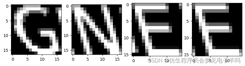
from skimage.measure import label, regionprops

def segment_image(image):
    labeled_image = label(image > 0)
    subimages = []
    for region in regionprops(labeled_image):
        start_x, start_y, end_x, end_y = region.bbox
        subimages.append(image[start_x:end_x, start_y:end_y])
    if len(subimages) == 0:
        return [image,]
    return subimages
subimages = segment_image(image)
f, axes = plt.subplots(1, len(subimages), figsize=(10, 3))
for i in range(len(subimages)):
    axes[i].imshow(subimages[i], cmap="gray")
from sklearn.utils import check_random_state
random_state = check_random_state(14)
letters = list("ACBDEFGHIJKLMNOPQRSTUVWXYZ")
shear_values = np.arange(0, 0.5, 0.05)
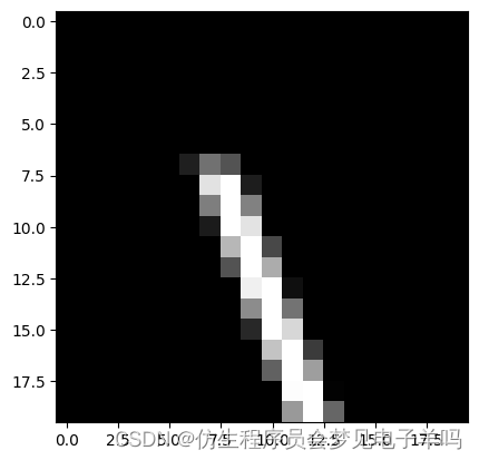
def generate_sample(random_state=None):
    random_state = check_random_state(random_state)
    letter = random_state.choice(letters)
    shear = random_state.choice(shear_values)
    return create_captcha(letter, shear=shear, size=(20, 20)), letters.index(letter)
image, target = generate_sample(random_state)
plt.imshow(image, cmap="gray")
print("The target for this image is: {0}".format(target))
The target for this image is: 11
dataset, targets = zip(*(generate_sample(random_state) for i in
range(3000)))
dataset = np.array(dataset, dtype='float')
targets = np.array(targets)
from sklearn.preprocessing import OneHotEncoder
onehot = OneHotEncoder()
y = onehot.fit_transform(targets.reshape(targets.shape[0],1))
y = y.todense()
from skimage.transform import resize
dataset = np.array([resize(segment_image(sample)[0], (20, 20)) for
sample in dataset])
X = dataset.reshape((dataset.shape[0], dataset.shape[1] *
dataset.shape[2]))
from sklearn.model_selection import train_test_split
X_train, X_test, y_train, y_test = \
train_test_split(X, y, train_size=0.9)
from pybrain.datasets import SupervisedDataSet
training = SupervisedDataSet(X.shape[1], y.shape[1])
for i in range(X_train.shape[0]):
    training.addSample(X_train[i], y_train[i])
testing = SupervisedDataSet(X.shape[1], y.shape[1])
for i in range(X_test.shape[0]):
    testing.addSample(X_test[i], y_test[i])
import scipy
from pybrain.tools.shortcuts import buildNetwork
net = buildNetwork(X.shape[1], 100, y.shape[1], bias=True)
from pybrain.supervised.trainers import BackpropTrainer
trainer = BackpropTrainer(net, training, learningrate=0.01,
weightdecay=0.01)
trainer.trainEpochs(epochs=20)
predictions = trainer.testOnClassData(dataset=testing)
下面这行代码micro部分是添加处理数据问题
from sklearn.metrics import f1_score
print("F-score: {0:.2f}".format(f1_score(predictions, y_test.argmax(axis=1), average='weighted')))
F-score: 0.89
from sklearn.metrics import classification_report
print(classification_report(y_test.argmax(axis=1), predictions))
              precision    recall  f1-score   support

           0       1.00      1.00      1.00         8
           1       0.72      1.00      0.84        13
           2       1.00      0.83      0.91        12
           3       1.00      1.00      1.00        12
           4       0.00      0.00      0.00        13
           5       0.41      1.00      0.58         9
           6       1.00      1.00      1.00        12
           7       1.00      1.00      1.00        12
           8       0.36      1.00      0.53         9
           9       0.00      0.00      0.00        10
          10       1.00      1.00      1.00        13
          11       0.33      0.14      0.20         7
          12       0.92      0.92      0.92        13
          13       0.95      1.00      0.98        20
          14       0.91      1.00      0.95        10
          15       0.90      1.00      0.95        19
          16       1.00      0.50      0.67        12
          17       1.00      1.00      1.00        13
          18       1.00      1.00      1.00        10
          19       1.00      1.00      1.00        11
          20       0.00      0.00      0.00         2
          21       1.00      0.93      0.96        14
          22       1.00      1.00      1.00        12
          23       1.00      1.00      1.00        13
          24       1.00      1.00      1.00         8
          25       1.00      1.00      1.00        13

    accuracy                           0.86       300
   macro avg       0.79      0.82      0.79       300
weighted avg       0.84      0.86      0.84       300
D:\coder\randomnumbers\venv\lib\site-packages\sklearn\metrics\_classification.py:1334: UndefinedMetricWarning: Precision and F-score are ill-defined and being set to 0.0 in labels with no predicted samples. Use `zero_division` parameter to control this behavior.
  _warn_prf(average, modifier, msg_start, len(result))
def predict_captcha(captcha_image, neural_network):
    subimages = segment_image(captcha_image)
    predicted_word = ""
    for subimage in subimages:
        subimage = resize(subimage, (20, 20))
        outputs = net.activate(subimage.flatten())
        prediction = np.argmax(outputs)
        predicted_word += letters[prediction]
    return predicted_word
word = "GENE"
captcha = create_captcha(word, shear=0.2)
print(predict_captcha(captcha, net))
ANAA
def test_prediction(word, net, shear=0.2):
    captcha = create_captcha(word, shear=shear)
    prediction = predict_captcha(captcha, net)
    prediction = prediction[:4]
    return word == prediction, word, prediction
from nltk.corpus import words
import nltk


valid_words = [word.upper() for word in words.words() if len(word) == 4]
num_correct = 0
num_incorrect = 0
for word in valid_words:
    correct, word, prediction = test_prediction(word, net, shear=0.2)
    if correct:
        num_correct += 1
    else:
        num_incorrect += 1
print("Number correct is {0}".format(num_correct))
print("Number incorrect is {0}".format(num_incorrect))
Number correct is 57
Number incorrect is 5456
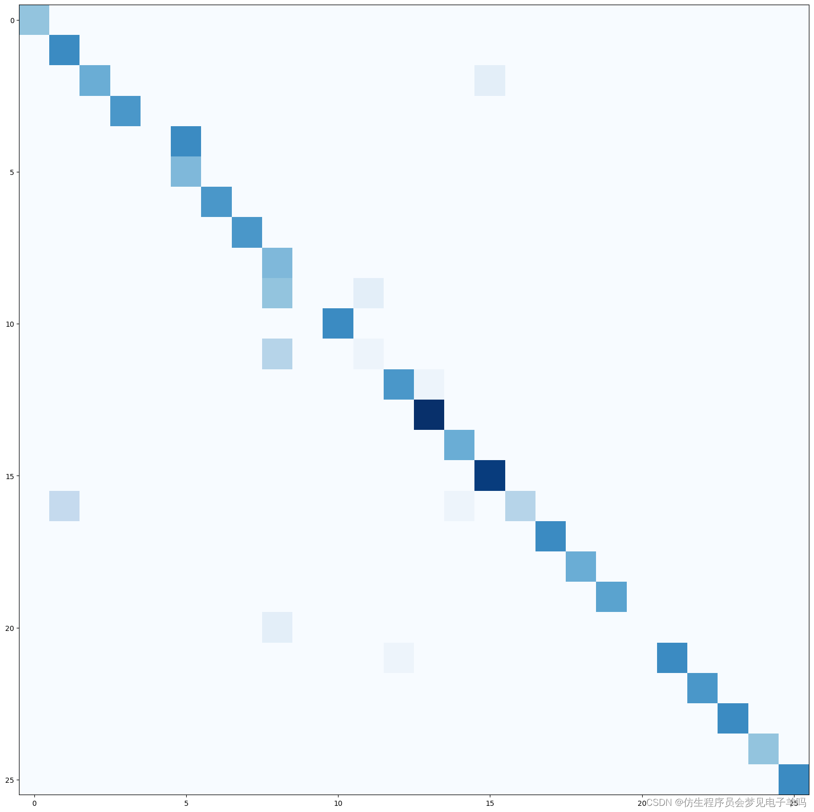
from sklearn.metrics import confusion_matrix
cm = confusion_matrix(np.argmax(y_test, axis=1), predictions)
plt.figure(figsize=(20,20))
plt.imshow(cm, cmap="Blues")
<matplotlib.image.AxesImage at 0x1b3ba7a4f40>
from nltk.metrics import edit_distance
steps = edit_distance("STEP", "STOP")
print("The number of steps needed is: {0}".format(steps))
The number of steps needed is: 1
def compute_distance(prediction, word):
    return len(prediction) - sum(prediction[i] == word[i] for i in range(len(prediction)))
from operator import itemgetter
def improved_prediction(word, net, dictionary, shear=0.2):
    captcha = create_captcha(word, shear=shear)
    prediction = predict_captcha(captcha, net)
    prediction = prediction[:4]
    if prediction not in dictionary:
        distances = sorted([(word, compute_distance(prediction, word))
                            for word in dictionary],
                           key=itemgetter(1))
        best_word = distances[0]
        prediction = best_word[0]
    return word == prediction, word, prediction
num_correct = 0
num_incorrect = 0
for word in valid_words:
    correct, word, prediction = improved_prediction (word, net, valid_words, shear=0.2)
    if correct:
        num_correct += 1
    else:
        num_incorrect += 1
print("Number correct is {0}".format(num_correct))
print("Number incorrect is {0}".format(num_incorrect))
Number correct is 123
Number incorrect is 5390