import numpy as np
import pandas as pd
import matplotlib.pyplot as plt
import torch
import warnings
warnings.filterwarnings('ignore')
%matplotlib inline
path = 'E:/nlp课件/test_data/temps.csv'
features = pd.read_csv(path)
features.head()
|
year |
month |
day |
week |
temp_2 |
temp_1 |
average |
actual |
friend |
| 0 |
2016 |
1 |
1 |
Fri |
45 |
45 |
45.6 |
45 |
29 |
| 1 |
2016 |
1 |
2 |
Sat |
44 |
45 |
45.7 |
44 |
61 |
| 2 |
2016 |
1 |
3 |
Sun |
45 |
44 |
45.8 |
41 |
56 |
| 3 |
2016 |
1 |
4 |
Mon |
44 |
41 |
45.9 |
40 |
53 |
| 4 |
2016 |
1 |
5 |
Tues |
41 |
40 |
46.0 |
44 |
41 |
数据表中
- year,moth,day,week分别表示的具体的时间
- temp_2:前天的最高温度值
- temp_1:昨天的最高温度值
- average:在历史中,每年这一天的平均最高温度值
- actual:标签值,当天的真实最高温度
print('数据维度:', features.shape)
数据维度: (348, 9)
# 处理时间
years = features['year']
month = features['month']
day = features['day']
dates = [str(int(years)) + '-' + str(int(month)) + '-' + str(int(day)) for years, month, day in zip(years, month, day)]
from datetime import datetime
dates = [datetime.strptime(date, '%Y-%m-%d') for date in dates]
dates[:5]
[datetime.datetime(2016, 1, 1, 0, 0),
 datetime.datetime(2016, 1, 2, 0, 0),
 datetime.datetime(2016, 1, 3, 0, 0),
 datetime.datetime(2016, 1, 4, 0, 0),
 datetime.datetime(2016, 1, 5, 0, 0)]
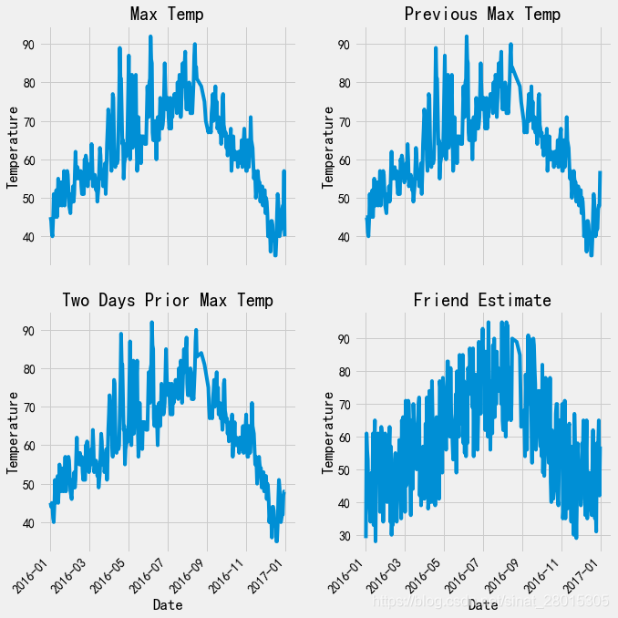
# 生成图像
# 默认风格
plt.style.use('fivethirtyeight')
# 设置布局
fig, ((ax1, ax2), (ax3, ax4)) = plt.subplots(nrows = 2, ncols = 2, figsize = (10,10))
fig.autofmt_xdate(rotation = 45)

# 标签值
ax1.plot(dates, features['actual'])
ax1.set_xlabel(''); ax1.set_ylabel('Temperature'); ax1.set_title('Max Temp')

# 昨天
ax2.plot(dates, features['temp_1'])
ax2.set_xlabel(''); ax2.set_ylabel('Temperature'); ax2.set_title('Previous Max Temp')

# 前天
ax3.plot(dates, features['temp_2'])
ax3.set_xlabel('Date'); ax3.set_ylabel('Temperature'); ax3.set_title('Two Days Prior Max Temp')

# 我的逗逼朋友
ax4.plot(dates, features['friend'])
ax4.set_xlabel('Date'); ax4.set_ylabel('Temperature'); ax4.set_title('Friend Estimate')

plt.tight_layout(pad=2)
# one-hot
features = pd.get_dummies(features)
features[:5]
|
year |
month |
day |
temp_2 |
temp_1 |
average |
actual |
friend |
week_Fri |
week_Mon |
week_Sat |
week_Sun |
week_Thurs |
week_Tues |
week_Wed |
| 0 |
2016 |
1 |
1 |
45 |
45 |
45.6 |
45 |
29 |
1 |
0 |
0 |
0 |
0 |
0 |
0 |
| 1 |
2016 |
1 |
2 |
44 |
45 |
45.7 |
44 |
61 |
0 |
0 |
1 |
0 |
0 |
0 |
0 |
| 2 |
2016 |
1 |
3 |
45 |
44 |
45.8 |
41 |
56 |
0 |
0 |
0 |
1 |
0 |
0 |
0 |
| 3 |
2016 |
1 |
4 |
44 |
41 |
45.9 |
40 |
53 |
0 |
1 |
0 |
0 |
0 |
0 |
0 |
| 4 |
2016 |
1 |
5 |
41 |
40 |
46.0 |
44 |
41 |
0 |
0 |
0 |
0 |
0 |
1 |
0 |
# 目标值
labels = np.array(features['actual'])

# 在特征之中去掉标签
features = features.drop('actual', axis = 1)

# 保存列名
features_list = list(features.columns)

# 转换格式
features = np.array(features)
features.shape
(348, 14)
from sklearn.preprocessing import StandardScaler
input_features = StandardScaler().fit_transform(features)
input_features[0]
array([ 0.        , -1.5678393 , -1.65682171, -1.48452388, -1.49443549,
       -1.3470703 , -1.98891668,  2.44131112, -0.40482045, -0.40961596,
       -0.40482045, -0.40482045, -0.41913682, -0.40482045])
构建网络模型
x = torch.tensor(input_features, dtype = float)
y = torch.tensor(labels, dtype = float)

# 权重参数初始化   [348,14] * [14, 128] * [128] * [128, 1] * [1]
weights = torch.randn((14, 128), dtype = float, requires_grad = True)
biases = torch.randn(128, dtype = float, requires_grad = True)
weights2 = torch.randn((128, 1), dtype = float, requires_grad = True)
biases2 = torch.randn(1, dtype = float, requires_grad = True)
learning_rate = 0.001
losses = []
for i in range(1000):
    # 计算隐层
    hidden = x.mm(weights) + biases
    # 激活函数
    hidden = torch.relu(hidden)
    # 预测结果
    predictions = hidden.mm(weights2) + biases2
    # 计算损失 - MSE
    loss = torch.mean((predictions - y)**2)
    losses.append(loss.data.numpy)

    # 打印损失
    if i % 100 == 0:
        print('loss:', loss)
    # 反向传播
    loss.backward()


    # 更新参数
    weights.data.add_(- learning_rate * weights.grad.data)
    biases.data.add_(- learning_rate * biases.grad.data)
    weights2.data.add_(- learning_rate * weights2)
    biases2.data.add_(- learning_rate * biases2)

    # 更新后梯度置0,否则会累加
    weights.grad.data.zero_()
    biases.grad.data.zero_()
    weights2.grad.data.zero_()
    biases2.grad.data.zero_()
loss: tensor(4769.2916, dtype=torch.float64, grad_fn=<MeanBackward0>)
loss: tensor(168.6445, dtype=torch.float64, grad_fn=<MeanBackward0>)
loss: tensor(152.0681, dtype=torch.float64, grad_fn=<MeanBackward0>)
loss: tensor(147.8071, dtype=torch.float64, grad_fn=<MeanBackward0>)
loss: tensor(146.4026, dtype=torch.float64, grad_fn=<MeanBackward0>)
loss: tensor(146.3492, dtype=torch.float64, grad_fn=<MeanBackward0>)
loss: tensor(147.1898, dtype=torch.float64, grad_fn=<MeanBackward0>)
loss: tensor(148.8380, dtype=torch.float64, grad_fn=<MeanBackward0>)
loss: tensor(151.3747, dtype=torch.float64, grad_fn=<MeanBackward0>)
loss: tensor(154.9829, dtype=torch.float64, grad_fn=<MeanBackward0>)
序列化容器构建网络模型
import torch.nn as nn
from torch.optim import Adam
input_size = input_features.shape[1]
hidden_size = 128
output_size = 1
batch_size = 16
my_nn = nn.Sequential(
    nn.Linear(input_size, hidden_size),
    nn.Sigmoid(),
    nn.Linear(hidden_size, output_size)
)
cost = nn.MSELoss(reduction= 'mean')
optimizer = Adam(my_nn.parameters(), lr = learning_rate)
# 训练网络
losses = []
for i in range(1000):
    batch_loss = []
    # mini_batch 方式进行训练
    for start in range(0, len(input_features), batch_size):
        end = start + batch_size if batch_size + start < len(input_features) else len(input_features)
        xx = torch.tensor(input_features[start : end], dtype = torch.float, requires_grad = True)
        yy = torch.tensor(labels[start : end], dtype = torch.float, requires_grad = True)
        # 前向传播
        predictions = my_nn(xx)
        # 计算损失
        loss = cost(predictions, yy)
        # 梯度置0
        optimizer.zero_grad()
        # 反向传播
        loss.backward(retain_graph = True)
        # 更新参数
        optimizer.step()

        batch_loss.append(loss.data.numpy())

    # 打印损失
    if i % 100 == 0:
        losses.append(np.mean(batch_loss))
        print(i, np.mean(batch_loss))
0 3980.642
100 37.847748
200 35.684933
300 35.318283
400 35.14371
500 35.006382
600 34.884396
700 34.761875
800 34.633102
900 34.49755
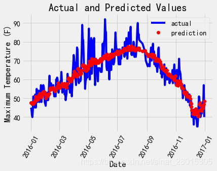
预测训练结果
x = torch.tensor(input_features, dtype = torch.float)
predict = my_nn(x).data.numpy()
# 转换日期格式
dates = [str(int(years)) + '-' + str(int(month)) + '-' + str(int(day)) for years, month, day in zip(years, month, day)]
dates = [datetime.strptime(date, '%Y-%m-%d') for date in dates]

# 创建一个表格来存日期和其对应的标签数值
true_data = pd.DataFrame(data = {'date': dates, 'actual': labels})

# 同理,再创建一个来存日期和其对应的模型预测值
months = features[:, features_list.index('month')]
days = features[:, features_list.index('day')]
years = features[:, features_list.index('year')]

test_dates = [str(int(year)) + '-' + str(int(month)) + '-' + str(int(day)) for year, month, day in zip(years, months, days)]

test_dates = [datetime.strptime(date, '%Y-%m-%d') for date in test_dates]

predictions_data = pd.DataFrame(data = {'date': test_dates, 'prediction': predict.reshape(-1)})
# 真实值
plt.plot(true_data['date'], true_data['actual'], 'b-', label = 'actual')

# 预测值
plt.plot(predictions_data['date'], predictions_data['prediction'], 'ro', label = 'prediction')
plt.xticks(rotation = '60');
plt.legend()

# 图名
plt.xlabel('Date'); plt.ylabel('Maximum Temperature (F)'); plt.title('Actual and Predicted Values');