欢迎关注笔者的微信公众号

如果使用matplotlib绘制论文图片时需要做非常多的设置,字体,大小,间距,多子图配置等,而这些操作可以封装好从而简化用户工作量。Proplot对matplotlib进行了封装和美化,用户可以使用与matplotlib相似的操作就画出更精美的图片。SciencePlots是matplotlib的样式库,内置了很多样式供用户选择,用它画出的图片可以满足出版的要求。
Proplot
要使用proplot绘图,必须先调用 figure 或 subplots 。这些是根据同名的 pyplot 命令建模的。跟matplotlib.pyplot 一样,subplots 一次创建一个图形和一个子图网格,而 figure 创建一个空图形,之后可以用子图填充。下面显示了一个只有一个子图的最小示例。
安装
pip install proplot
conda install -c conda-forge proplot
import numpy as np
import proplot as pplt
import warnings
warnings.filterwarnings('ignore')
state = np.random.RandomState(51423)
data = 2 * (state.rand(100, 5) - 0.5).cumsum(axis=0)
fig = pplt.figure()
ax = fig.subplot(121)
ax.plot(data, lw=2)
ax = fig.subplot(122)
fig.format(
suptitle='Simple subplot grid', title='Title',
xlabel='x axis', ylabel='y axis'
)

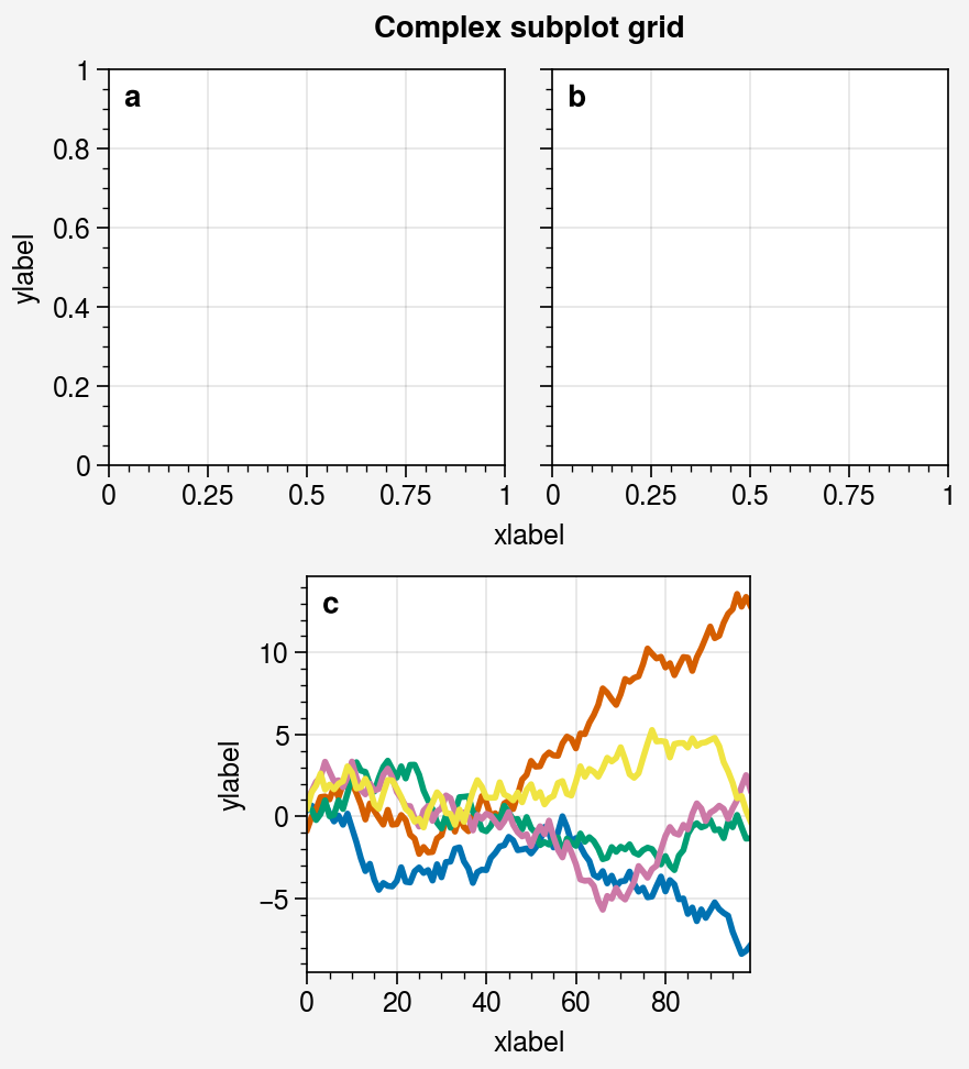
import numpy as np
import proplot as pplt
state = np.random.RandomState(51423)
data = 2 * (state.rand(100, 5) - 0.5).cumsum(axis=0)
array = [
[1, 1, 2, 2],
[0, 3, 3, 0],
]
fig = pplt.figure(refwidth=1.8)
axs = fig.subplots(array)
axs.format(
abc=True, abcloc='ul', suptitle='Complex subplot grid',
xlabel='xlabel', ylabel='ylabel'
)
axs[2].plot(data, lw=2)
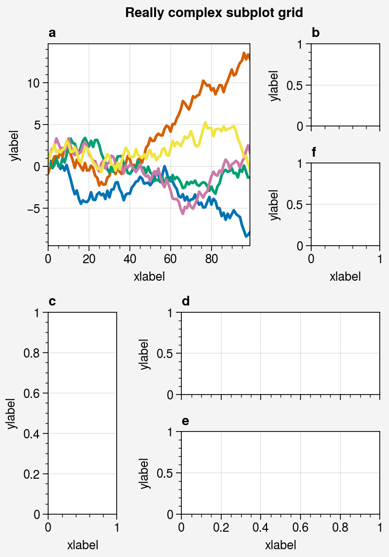
import numpy as np
import proplot as pplt
state = np.random.RandomState(51423)
data = 2 * (state.rand(100, 5) - 0.5).cumsum(axis=0)
array = [
[1, 1, 2],
[1, 1, 6],
[3, 4, 4],
[3, 5, 5],
]
fig, axs = pplt.subplots(array, figwidth=5, span=False)
axs.format(
suptitle='Really complex subplot grid',
xlabel='xlabel', ylabel='ylabel', abc=True
)
axs[0].plot(data, lw=2)
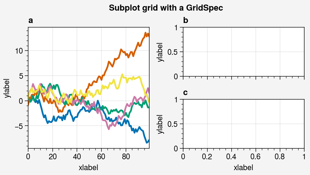
import numpy as np
import proplot as pplt
state = np.random.RandomState(51423)
data = 2 * (state.rand(100, 5) - 0.5).cumsum(axis=0)
gs = pplt.GridSpec(nrows=2, ncols=2, pad=1)
fig = pplt.figure(span=False, refwidth=2)
ax = fig.subplot(gs[:, 0])
ax.plot(data, lw=2)
ax = fig.subplot(gs[0, 1])
ax = fig.subplot(gs[1, 1])
fig.format(
suptitle='Subplot grid with a GridSpec',
xlabel='xlabel', ylabel='ylabel', abc=True
)
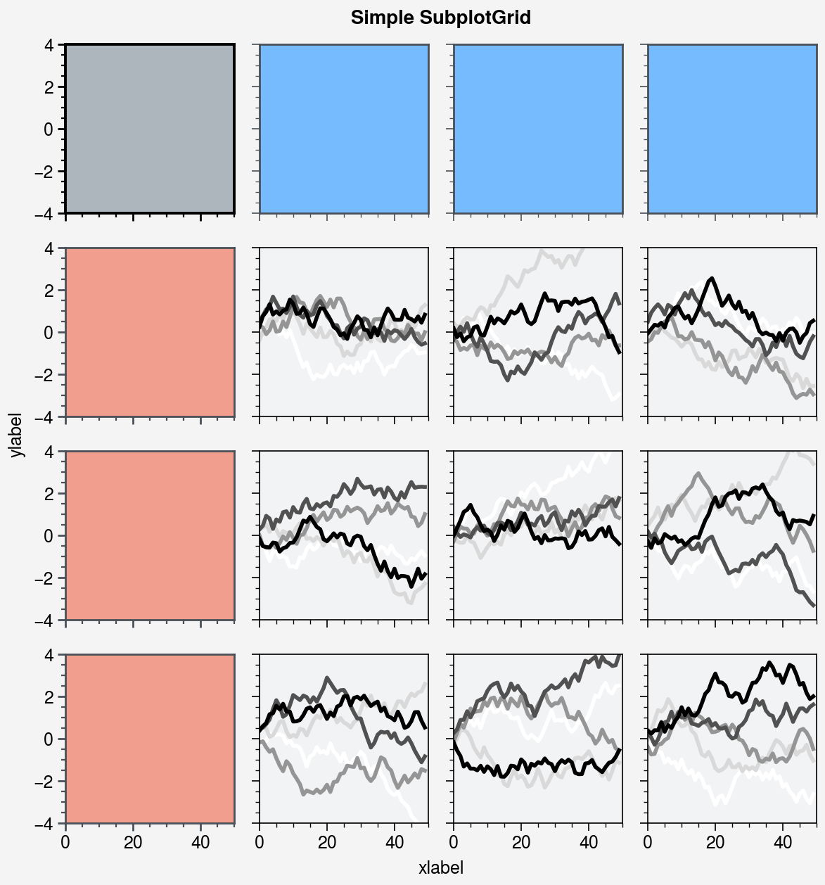
import proplot as pplt
import numpy as np
state = np.random.RandomState(51423)
fig, axs = pplt.subplots(ncols=4, nrows=4, refwidth=1.2, span=True)
axs.format(xlabel='xlabel', ylabel='ylabel', suptitle='Simple SubplotGrid')
axs.format(grid=False, xlim=(0, 50), ylim=(-4, 4))
axs[:, 0].format(facecolor='blush', edgecolor='gray7', linewidth=1)
axs[:, 0].format(fc='blush', ec='gray7', lw=1)
axs[0, :].format(fc='sky blue', ec='gray7', lw=1)
axs[0].format(ec='black', fc='gray5', lw=1.4)
axs[1:, 1:].format(fc='gray1')
for ax in axs[1:, 1:]:
ax.plot((state.rand(50, 5) - 0.5).cumsum(axis=0), cycle='Grays', lw=2)
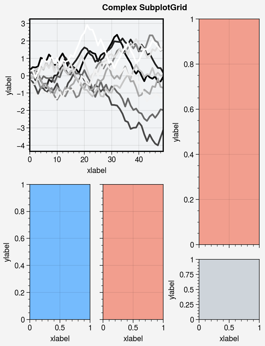
fig = pplt.figure(refwidth=1, refnum=5, span=False)
axs = fig.subplots([[1, 1, 2], [3, 4, 2], [3, 4, 5]], hratios=[2.2, 1, 1])
axs.format(xlabel='xlabel', ylabel='ylabel', suptitle='Complex SubplotGrid')
axs[0].format(ec='black', fc='gray1', lw=1.4)
axs[1, 1:].format(fc='blush')
axs[1, :1].format(fc='sky blue')
axs[-1, -1].format(fc='gray4', grid=False)
axs[0].plot((state.rand(50, 10) - 0.5).cumsum(axis=0), cycle='Grays_r', lw=2)
import proplot as pplt
import numpy as np
N = 20
state = np.random.RandomState(51423)
data = N + (state.rand(N, N) - 0.55).cumsum(axis=0).cumsum(axis=1)
cycle = pplt.Cycle('greys', left=0.2, N=5)
fig, axs = pplt.subplots(ncols=2, nrows=2, figwidth=5, share=False)
axs[0].plot(data[:, :5], linewidth=2, linestyle='--', cycle=cycle)
axs[1].scatter(data[:, :5], marker='x', cycle=cycle)
axs[2].pcolormesh(data, cmap='greys')
m = axs[3].contourf(data, cmap='greys')
axs.format(
abc='a.', titleloc='l', title='Title',
xlabel='xlabel', ylabel='ylabel', suptitle='Quick plotting demo'
)
fig.colorbar(m, loc='b', label='label')

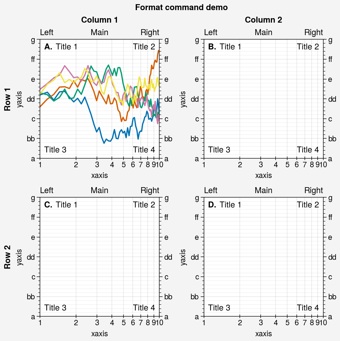
import proplot as pplt
import numpy as np
fig, axs = pplt.subplots(ncols=2, nrows=2, refwidth=2, share=False)
state = np.random.RandomState(51423)
N = 60
x = np.linspace(1, 10, N)
y = (state.rand(N, 5) - 0.5).cumsum(axis=0)
axs[0].plot(x, y, linewidth=1.5)
axs.format(
suptitle='Format command demo',
abc='A.', abcloc='ul',
title='Main', ltitle='Left', rtitle='Right',
ultitle='Title 1', urtitle='Title 2', lltitle='Title 3', lrtitle='Title 4',
toplabels=('Column 1', 'Column 2'),
leftlabels=('Row 1', 'Row 2'),
xlabel='xaxis', ylabel='yaxis',
xscale='log',
xlim=(1, 10), xticks=1,
ylim=(-3, 3), yticks=pplt.arange(-3, 3),
yticklabels=('a', 'bb', 'c', 'dd', 'e', 'ff', 'g'),
ytickloc='both', yticklabelloc='both',
xtickdir='inout', xtickminor=False, ygridminor=True,
)
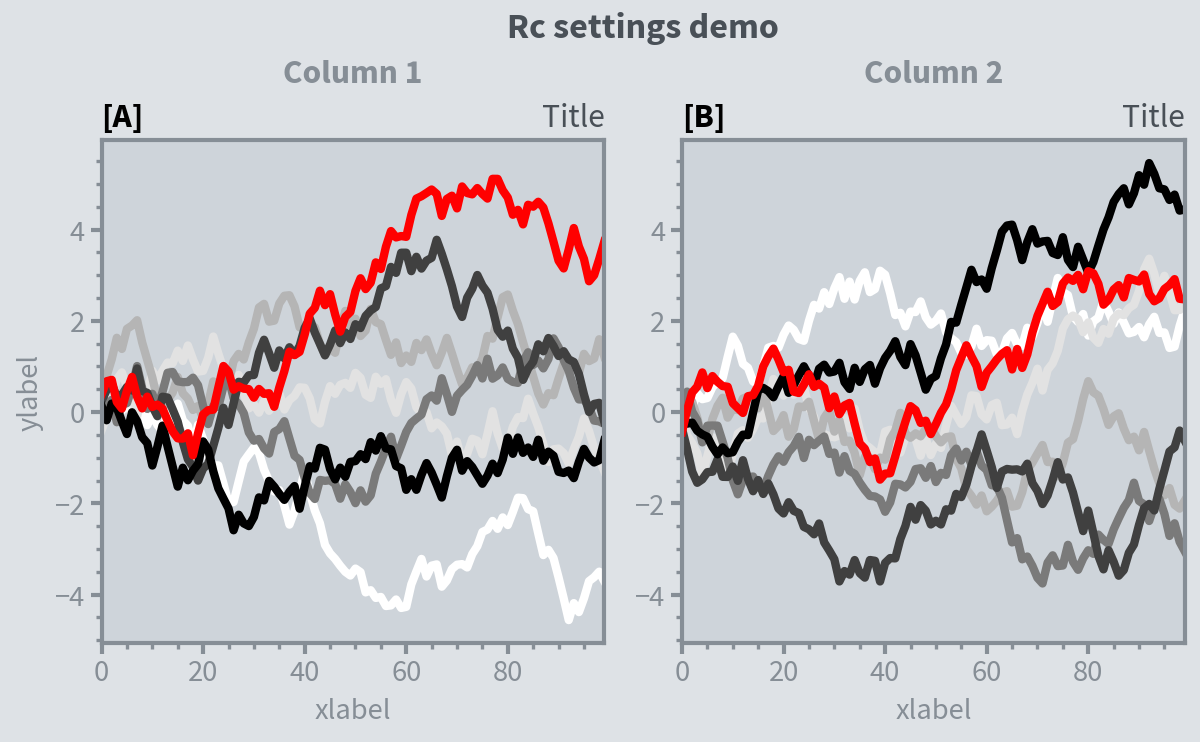
import proplot as pplt
import numpy as np
pplt.rc.metacolor = 'gray6'
pplt.rc.update({'fontname': 'Source Sans Pro', 'fontsize': 11})
pplt.rc['figure.facecolor'] = 'gray3'
pplt.rc.axesfacecolor = 'gray4'
with pplt.rc.context({'suptitle.size': 13}, toplabelcolor='gray6', metawidth=1.5):
fig = pplt.figure(figwidth=6, sharey='limits', span=False)
axs = fig.subplots(ncols=2)
N, M = 100, 7
state = np.random.RandomState(51423)
values = np.arange(1, M + 1)
cycle = pplt.get_colors('grays', M - 1) + ['red']
for i, ax in enumerate(axs):
data = np.cumsum(state.rand(N, M) - 0.5, axis=0)
lines = ax.plot(data, linewidth=3, cycle=cycle)
axs.format(
grid=False, xlabel='xlabel', ylabel='ylabel',
toplabels=('Column 1', 'Column 2'),
suptitle='Rc settings demo',
suptitlecolor='gray7',
abc='[A]', abcloc='l',
title='Title', titleloc='r', titlecolor='gray7'
)
pplt.rc.reset()
import proplot as pplt
import numpy as np
state = np.random.RandomState(51423)
data = state.rand(10, 5)
fig, axs = pplt.subplots(ncols=2, nrows=2, span=False, share=False)
axs.format(suptitle='Stylesheets demo')
styles = ('ggplot', 'seaborn', '538', 'bmh')
for ax, style in zip(axs, styles):
ax.format(style=style, xlabel='xlabel', ylabel='ylabel', title=style)
ax.plot(data, linewidth=3)

SciencePlots
安装
pip install SciencePlots
pip install git+https://github.com/garrettj403/SciencePlots
git clone https://github.com/garrettj403/SciencePlots.git
cd SciencePlots
pip install -e .
根据系统不同,需要提前安装latex环境
例子
import numpy as np
import matplotlib
import matplotlib.pyplot as plt
matplotlib.style.reload_library()
matplotlib.rcParams['axes.unicode_minus'] = False
def model(x, p):
return x ** (2 * p + 1) / (1 + x ** (2 * p))
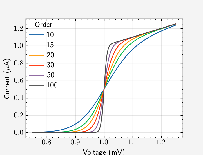
pparam = dict(xlabel='Voltage (mV)', ylabel='Current ($\mu$A)')
x = np.linspace(0.75, 1.25, 201)
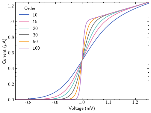
with plt.style.context(['science']):
fig, ax = plt.subplots()
for p in [10, 15, 20, 30, 50, 100]:
ax.plot(x, model(x, p), label=p)
ax.legend(title='Order')
ax.set(**pparam)
fig.savefig('figures/fig1.jpg', dpi=300)
with plt.style.context(['science', 'ieee', 'notebook']):
fig, ax = plt.subplots()
for p in [10, 20, 40, 100]:
ax.plot(x, model(x, p), label=p)
ax.legend(title='Order')
ax.autoscale(tight=True)
ax.set(**pparam)
ax.set_ylabel(r'$Current (\mu A)$')
fig.savefig('figures/fig2a.jpg', dpi=300)

with plt.style.context(['science', 'ieee', 'std-colors', 'notebook']):
fig, ax = plt.subplots()
for p in [10, 15, 20, 30, 50, 100]:
ax.plot(x, model(x, p), label=p)
ax.legend(title='Order')
ax.autoscale(tight=True)
ax.set(**pparam)
ax.set_ylabel(r'$Current (\mu A)$')
fig.savefig('figures/fig2b.jpg', dpi=300)
with plt.style.context(['science', 'high-vis', 'notebook']):
fig, ax = plt.subplots()
for p in [10, 15, 20, 30, 50, 100]:
ax.plot(x, model(x, p), label=p)
ax.legend(title='Order')
ax.autoscale(tight=True)
ax.set(**pparam)
fig.savefig('figures/fig4.jpg', dpi=300)
with plt.style.context(['dark_background', 'science', 'high-vis', 'notebook']):
fig, ax = plt.subplots()
for p in [10, 15, 20, 30, 50, 100]:
ax.plot(x, model(x, p), label=p)
ax.legend(title='Order')
ax.autoscale(tight=True)
ax.set(**pparam)
fig.savefig('figures/fig5.jpg', dpi=300)
with plt.style.context(['science', 'notebook']):
fig, ax = plt.subplots()
for p in [10, 15, 20, 30, 50, 100]:
ax.plot(x, model(x, p), label=p)
ax.legend(title='Order')
ax.autoscale(tight=True)
ax.set(**pparam)
fig.savefig('figures/fig10.jpg', dpi=300)

with plt.style.context(['science', 'bright', 'notebook']):
fig, ax = plt.subplots()
for p in [5, 10, 15, 20, 30, 50, 100]:
ax.plot(x, model(x, p), label=p)
ax.legend(title='Order')
ax.autoscale(tight=True)
ax.set(**pparam)
fig.savefig('figures/fig6.jpg', dpi=300)

with plt.style.context(['science', 'muted', 'notebook']):
fig, ax = plt.subplots()
for p in [5, 7, 10, 15, 20, 30, 38, 50, 100, 500]:
ax.plot(x, model(x, p), label=p)
ax.legend(title='Order', fontsize=7)
ax.autoscale(tight=True)
ax.set(**pparam)
fig.savefig('figures/fig8.jpg', dpi=300)

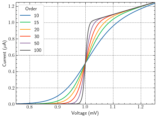
with plt.style.context(['science', 'grid', 'notebook']):
fig, ax = plt.subplots()
for p in [10, 15, 20, 30, 50, 100]:
ax.plot(x, model(x, p), label=p)
ax.legend(title='Order')
ax.autoscale(tight=True)
ax.set(**pparam)
fig.savefig('figures/fig11.jpg', dpi=300)
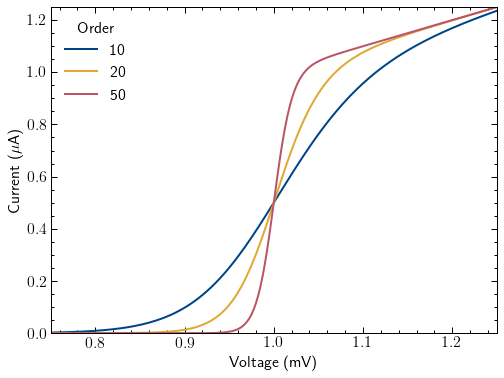
with plt.style.context(['science', 'high-contrast', 'notebook']):
fig, ax = plt.subplots()
for p in [10, 20, 50]:
ax.plot(x, model(x, p), label=p)
ax.legend(title='Order')
ax.autoscale(tight=True)
ax.set(**pparam)
fig.savefig('figures/fig12.jpg', dpi=300)
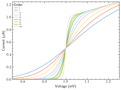
with plt.style.context(['science', 'light', 'notebook']):
fig, ax = plt.subplots()
for p in [5, 7, 10, 15, 20, 30, 38, 50, 100]:
ax.plot(x, model(x, p), label=p)
ax.legend(title='Order', fontsize=7)
ax.autoscale(tight=True)
ax.set(**pparam)
fig.savefig('figures/fig13.jpg', dpi=300)
参考资料
- https://proplot.readthedocs.io
- https://github.com/garrettj403/SciencePlots
本文内容由网友自发贡献,版权归原作者所有,本站不承担相应法律责任。如您发现有涉嫌抄袭侵权的内容,请联系:hwhale#tublm.com(使用前将#替换为@)