????????????????
欢迎来到本博客
❤️❤️????????
????博主优势:
????????????
博客内容尽量做到思维缜密,逻辑清晰,为了方便读者。
⛳️
座右铭:
行百里者,半于九十。
????????????
本文目录如下:
????????????
目录
????1 概述
????2 运行结果
????3 参考文献
????4 Python代码及文章
????1 概述
文献来源:

摘要:
具有恒温控制的负载,如冰箱,非常适合作为灵活的需求资源。本文提出了一种用于冰箱的分散式负载控制算法。该算法改编自现有的连续时间控制方法,旨在实现低计算复杂性和处理可变长度离散时间步骤的能力,这些是嵌入在电器和高吞吐量模拟中的理想特性。大量异质电器的模拟结果说明了对功耗的准确集中控制和高计算效率。冰箱和其他恒温控制负载的物理特性使它们非常适合作为向电网提供灵活性的低成本提供者:它们的功耗可以在十几分钟内移位而不会对冷却性能产生明显影响。这种灵活性可以用于提供响应和储备服务,以减少极端负载水平并缓解爬坡约束[1]。鉴于涉及的设备数量庞大,可以使用随机控制方案有效地分散控制大规模电器群体,如[2]–[4]中提出的。实际实施还必须考虑实施、计算和通信方面的约束,如[5]、[6]中所讨论的。
在[7]中引入了一种用于异质TCL的健壮分散式控制方案,并在[8]中进行了扩展,以允许TCL集体从电网吸收能量的情景。该控制策略具有令人满意的特性,即它只需要单向广播信息,但可以实现对预期参考信号的跟踪(即对大量设备来说是精确的),而不违反各个设备的温度限制。然而,其连续时间形式的积分形式不利于在嵌入式控制器上实施或者同时快速模拟多个设备。本文通过推导一种离散时间控制算法来解决这一缺点,该算法实施了[7]、[8]中提出的控制策略。该算法特别适用于具有计算约束的设备上的实施。具体而言,它避免了数值积分,并使用可变大小的贪婪时间步长,以便放宽实时性能要求。首先,描述了一个离散化过程,针对分段常数控制信号的情况,并重新构造了控制器的自然坐标。然后,推导出了控制设备行为的每个开关过程的表达式。最后,提供了一个明确的控制算法,并利用基于Python的模拟展示了其对异质冰箱群体的有效性。
????
2 运行结果
# Two subplots, the axes array is 1-d
fig, axarr = plt.subplots(2, sharex=True)
axarr[0].plot(time_list/3600,70*dcycles.mean() * np.array(pi_profile),'k', label='$\Pi$')
axarr[0].plot(time_list/3600,70*results.mean(axis=0),'r',label='100k')
axarr[0].plot(time_list/3600,70*results1k.mean(axis=0), label='1k')
axarr[0].legend(loc='lower right')

axarr[1].plot(time_list/3600,70*(results.mean(axis=0)- dcycles.mean() * np.array(pi_profile)),'r',label='100k')
axarr[1].plot(time_list/3600,70*(results1k.mean(axis=0)- dcycles1k.mean() * np.array(pi_profile)),label='1k')
axarr[1].legend(loc='lower right')

#plt.axes().set_aspect(1)
fig.set_size_inches(3.5,3.5)
axarr[1].set_xlabel('time [h]')
axarr[0].set_ylabel('consumption \nper appliance [W]')
axarr[1].set_ylabel('deviation \nper appliance [W]')

plt.plot(z_list)

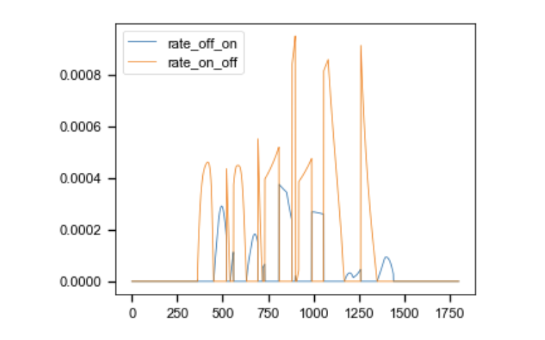
plt.plot(rate1_list, label='rate_off_on')
plt.plot(rate2_list, label='rate_on_off')
plt.legend()
# Two subplots, the axes array is 1-d
fig, axarr = plt.subplots(3, sharex=True)
axarr[0].plot(time_list/3600, pi_profile,'k')
axarr[1].plot(time_list/3600, control_list,'k')
axarr[2].plot(time_list/3600, temperature_list,'k')

fig.set_size_inches(3.5,3.5)
axarr[2].set_xlabel('time [h]')
axarr[0].set_ylabel('reference $\Pi$')
axarr[0].set_ylim((0.5,1.5))
axarr[1].set_ylabel('control state $c$')
axarr[2].set_ylabel('temperature [${}^\circ C$]')

pi_profile1 = np.array([1.0 for time in time_list_small])
pi_profile2 = np.array([1.0 + 0.3 * np.sin(2*np.pi*time/1800) for time in time_list_small])
pi_profile3 = np.array([1.0 + 0.3 * signal.square(2*np.pi*time/1800) for time in time_list_small])
pi_profile4 = np.array([1.0 + 0.3 * signal.sawtooth(2*np.pi*time/1800) for time in time_list_small])

pi_profile = np.concatenate((pi_profile1, pi_profile2, pi_profile3, pi_profile4, pi_profile1))

plt.plot(time_list/3600, pi_profile)
plt.gca().set_xlabel('hours');
plt.gca().set_ylabel('$\Pi$');

????3
参考文献
文章中一些内容引自网络,会注明出处或引用为参考文献,难免有未尽之处,如有不妥,请随时联系删除。

????
4 Python代码及文章