导入需要的库
import matplotlib.pyplot as plt
import numpy as np
from jupyterthemes import jtplot
jtplot.style(grid=False)
建立xy对应关系
x = np.linspace(-2, np.pi)
y1 = np.sin(x)
y2 = np.cos(x)
plot()
matplotlib.pyplot.plot()参数详解
https://matplotlib.org/api/pyplot_summary.html
#单条线:
plot([x], y, [fmt], data=None, **kwargs)
#多条线一起画
plot([x], y, [fmt], [x2], y2, [fmt2], …, **kwargs)
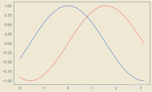
plt.figure(num=2,figsize=(8,5))
plt.plot(x,y2)
plt.plot(x,y1,color='red',linewidth=1.0,linestyle='--')
plt.show()
plt.xlim(), plt.ylim()
确定显示的xy范围
plt.figure(num=2,figsize=(8,5))
plt.plot(x,y2)
plt.plot(x,y1,color='red',linewidth=1.0,linestyle='--')
plt.xlim((-1,2))
plt.ylim((-2,3))
plt.xlabel('I am x')
plt.ylabel('I am y')
plt.savefig("1.png")
plt.show()
修改x, y轴的标签
new_ticks = np.linspace(-1,2,5)
plt.xticks(new_ticks)
plt.yticks([-2,-1.8,-1,1.22,3],[r’
n
n
n’,r’
n
r
nr
nr’,r’
s
s
s’,r’
s
r
sr
sr’,r’
s
s
r
ssr
ssr’])
plt.figure(num=3,figsize=(8,5))
plt.plot(x,y2)
plt.plot(x,y1,color='red',linewidth=1.0,linestyle='--')
plt.xlim((-1,2))
plt.ylim((-2,3))
plt.xlabel('I am x')
plt.ylabel('I am y')
new_ticks = np.linspace(-1,2,5)
plt.xticks(new_ticks)
plt.yticks([-2,-1.8,-1,1.22,3],[r'$n$',r'$nr$',r'$s$',r'$sr$',r'$ssr$'])
plt.show()
修改边框
ax = plt.gca()
ax.spines[‘你想要修改的边’].set_color(‘none’)
修改坐标轴位置
ax.xaxis.set_ticks_position(‘bottom’)
ax.spines[‘bottom’].set_position((‘data’,0))
ax.yaxis.set_ticks_position(‘left’)
ax.spines[‘left’].set_position((‘data’,0))
plt.figure(num=3,figsize=(8,5))
plt.plot(x,y2)
plt.plot(x,y1,color='red',linewidth=1.0,linestyle='--')
plt.xlim((-1,2))
plt.ylim((-2,3))
plt.xlabel('I am x')
plt.ylabel('I am y')
new_ticks = np.linspace(-1,2,5)
plt.xticks(new_ticks)
plt.yticks([-2,-1.8,-1,1.22,3],[r'$n$',r'$nr$',r'$s$',r'$sr$',r'$ssr$'])

ax = plt.gca()
ax.spines['right'].set_color('none')
ax.spines['top'].set_color('none')

ax.xaxis.set_ticks_position('bottom')
ax.spines['bottom'].set_position(('data',0))

ax.yaxis.set_ticks_position('left')
ax.spines['left'].set_position(('data',0))

plt.show()
小练习
import matplotlib.pyplot as plt
import numpy as np
from jupyterthemes import jtplot
jtplot.style(grid=False)
plt.style.use(plt.style.available[1])
plt.rcParams['font.family'] = ['sans-serif']
plt.rcParams['font.sans-serif'] = ['SimHei']
plt.rcParams['axes.unicode_minus']=False
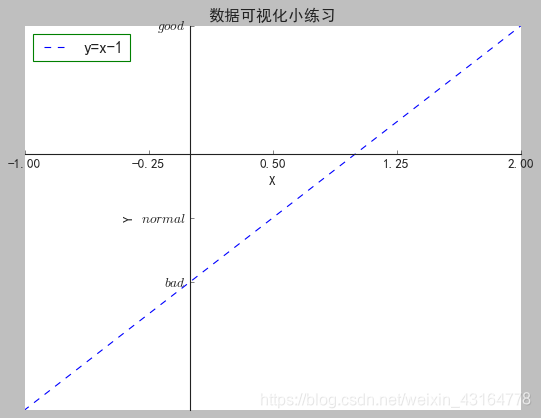
x = np.linspace(-2, 3)
y = x-1
plt.plot(x,y,color='blue',linewidth=1.0,linestyle='--',label='y=x-1')
plt.xlim((-1,2))
plt.ylim((-2,1))
plt.xlabel('X')
plt.ylabel('Y')
new_ticks = np.linspace(-1,2,5)
plt.xticks(new_ticks)
plt.yticks([-1,-0.5,1],[r'$bad$',r'$normal$',r'$good$'])
ax = plt.gca()
ax.spines['right'].set_color('none')
ax.spines['top'].set_color('none')
ax.xaxis.set_ticks_position('bottom')
ax.spines['bottom'].set_position(('data',0))
ax.yaxis.set_ticks_position('left')
ax.spines['left'].set_position(('data',0))
plt.title(r'数据可视化小练习')
plt.legend(loc='best',edgecolor='green')
plt.savefig("数据可视化.png")
plt.show()
Annotation 标注
当图线中某些特殊地方需要标注时,我们可以使用 annotation. matplotlib 中的 annotation 有两种方法,一种是用 plt 里面的 annotate,一种是直接用 plt 里面的 text 来写标注。首先回顾一下上一章节的画图教程:
x = np.linspace(-3, 3, 50)
y = 2*x + 1
plt.figure(num=1, figsize=(8, 5),)
ax = plt.gca()
ax.spines['right'].set_color('none')
ax.spines['top'].set_color('none')
ax.spines['top'].set_color('none')
ax.xaxis.set_ticks_position('bottom')
ax.spines['bottom'].set_position(('data', 0))
ax.yaxis.set_ticks_position('left')
ax.spines['left'].set_position(('data', 0))
plt.plot(x, y,)
x0 = 1
y0 = 2*x0 + 1
plt.plot([x0, x0,], [0, y0,], 'k--', linewidth=2.5)
plt.scatter([x0, ], [y0, ], s=50, color='b')
<matplotlib.collections.PathCollection at 0x1bf13d48ac8>

添加注释 annotate
接下来我们就对(x0, y0)这个点进行标注。第一种方式就是利用函数 annotate(),其中 r’’ %y0 代表标注的内容,可以通过字符串 %s 将 y0 的值传入字符串;参数xycoords=‘data’ 是说基于数据的值来选位置, xytext=(+30, -30) 和 textcoords=‘offset points’ 表示对于标注位置的描述 和 xy 偏差值,即标注位置是 xy 位置向右移动 30,向下移动30, arrowprops是对图中箭头类型和箭头弧度的设置,需要用 dict 形式传入。
plt.figure(num=1, figsize=(8, 5),)
ax = plt.gca()
ax.spines['right'].set_color('none')
ax.spines['top'].set_color('none')
ax.spines['top'].set_color('none')
ax.xaxis.set_ticks_position('bottom')
ax.spines['bottom'].set_position(('data', 0))
ax.yaxis.set_ticks_position('left')
ax.spines['left'].set_position(('data', 0))
plt.plot(x, y,)
x0 = 1
y0 = 2*x0 + 1
plt.plot([x0, x0,], [0, y0,], 'k--', linewidth=2.5)
plt.scatter([x0, ], [y0, ], s=50, color='b')
plt.annotate(r'$2x+1=%s$' % y0, xy=(x0, y0), xycoords='data', xytext=(+30, -30),
textcoords='offset points', fontsize=16,
arrowprops=dict(arrowstyle='->', connectionstyle="arc3,rad=.2"))
Text(30,-30,'$2x+1=3$')
![(img-4fXVKph6-1601519009565)(output_17_1.png)]](https://img-blog.csdnimg.cn/20201001103025840.png?x-oss-process=image/watermark,type_ZmFuZ3poZW5naGVpdGk,shadow_10,text_aHR0cHM6Ly9ibG9nLmNzZG4ubmV0L3dlaXhpbl80MzE2NDc3OA==,size_16,color_FFFFFF,t_70#pic_center)
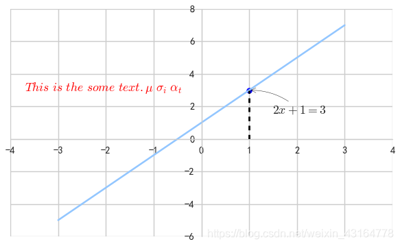
添加注释 text
第二种注释方式是通过text()函数
plt.figure(num=1, figsize=(8, 5),)
ax = plt.gca()
ax.spines['right'].set_color('none')
ax.spines['top'].set_color('none')
ax.spines['top'].set_color('none')
ax.xaxis.set_ticks_position('bottom')
ax.spines['bottom'].set_position(('data', 0))
ax.yaxis.set_ticks_position('left')
ax.spines['left'].set_position(('data', 0))
plt.plot(x, y,)
x0 = 1
y0 = 2*x0 + 1
plt.plot([x0, x0,], [0, y0,], 'k--', linewidth=2.5)
plt.scatter([x0, ], [y0, ], s=50, color='b')
plt.annotate(r'$2x+1=%s$' % y0, xy=(x0, y0), xycoords='data', xytext=(+30, -30),
textcoords='offset points', fontsize=16,
arrowprops=dict(arrowstyle='->', connectionstyle="arc3,rad=.2"))
plt.text(-3.7, 3, r'$This\ is\ the\ some\ text. \mu\ \sigma_i\ \alpha_t$',
fontdict={'size': 16, 'color': 'r'})
Text(-3.7,3,'$This\\ is\\ the\\ some\\ text. \\mu\\ \\sigma_i\\ \\alpha_t$')
plt.figure(num=3,figsize=(8,5))
plt.plot(x,y2,label='cos x')
plt.plot(x,y1,color='red',linewidth=1.0,linestyle='--',label='sin x')
plt.xlim((-1,2))
plt.ylim((-2,3))
plt.xlabel('I am x')
plt.ylabel('I am y')
new_ticks = np.linspace(-1,2,5)
plt.xticks(new_ticks)
plt.yticks([-2,-1.8,-1,1.22,3],[r'$n$',r'$nr$',r'$s$',r'$sr$',r'$ssr$'])

ax = plt.gca()
ax.spines['right'].set_color('none')
ax.spines['top'].set_color('none')

ax.xaxis.set_ticks_position('bottom')
ax.spines['bottom'].set_position(('data',0))

ax.yaxis.set_ticks_position('left')
ax.spines['left'].set_position(('data',0))

plt.legend(loc='best',edgecolor='brown')

plt.show()

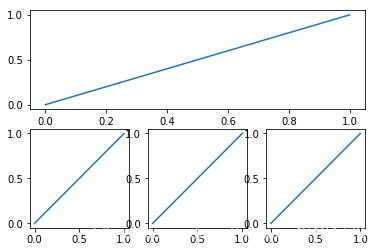
plt.subplot(2,1,1)
plt.plot([0,1],[0,1])

plt.subplot(2,3,4)
plt.plot([0,1],[0,1])

plt.subplot(2,3,5)
plt.plot([0,1],[0,1])

plt.subplot(2,3,6)
plt.plot([0,1],[0,1])
[<matplotlib.lines.Line2D at 0x223d1011748>]
ax1 = plt.subplot2grid((3,3),(0,0),colspan=3)
ax1.plot([1,2],[1,2])
ax1.set_title('ax1_title')

ax2 = plt.subplot2grid((3,3),(1,0),colspan=2)

ax3 = plt.subplot2grid((3,3),(1,2),rowspan=3)

ax4 = plt.subplot2grid((3,3),(2,0))

ax5 = plt.subplot2grid((3,3),(2,1))

ax4.scatter([1,2],[2,2])
ax4.set_xlabel('ax4_x')
ax4.set_ylabel('ax4_y')
Text(0,0.5,'ax4_y')

f,((ax11,ax12),(ax13,ax14)) = plt.subplots(2,2,sharex=True,sharey=True)
ax11.scatter([1,2], [1,2])
<matplotlib.collections.PathCollection at 0x20fe72b4358>

使用同一刻度线
twinx()函数表示共享x轴
twiny()表示共享y轴
共享表示的就是x轴使用同一刻度线
python—之suplot里面的twinx()函数
ax2 = ax1.twinx()
fig,ax1 = plt.subplots()
ax2 = ax1.twinx()
ax1.plot(x,y1,‘g-’)
ax1.set_xlabel(‘X data’)
ax1.set_ylabel(‘Y1 data’, color=‘g’)
ax2.plot(x, y2, ‘b-’) # blue
ax2.set_ylabel(‘Y2 data’, color=‘b’)
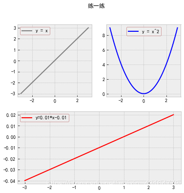
练一练
方法一 plt.subplot
plt.style.use(plt.style.available[0])
plt.rcParams['font.family'] = ['sans-serif']
plt.rcParams['font.sans-serif'] = ['SimHei']
plt.rcParams['axes.unicode_minus']=False
plt.figure(figsize=(6,6))
plt.suptitle('练一练')
x = np.linspace(-3, 3)
y = x
plt.subplot(2,2,1)
plt.plot(x,y,label='y = x',color='grey')
plt.legend(loc='best',edgecolor='brown')
y = x**2
plt.subplot(2,2,2)
plt.plot(x,y,label='y = x^2',color='b')
plt.legend(loc='best',edgecolor='brown')
y = 0.01*x - 0.01
plt.subplot(2,1,2)
plt.plot(x,y,label='y=0.01*x-0.01',color='r')
plt.legend(loc='best',edgecolor='brown')
<matplotlib.legend.Legend at 0x1bf0f1b41d0>
方法二 plt.subplots
plt.style.use(plt.style.available[21])
plt.rcParams['font.family'] = ['sans-serif']
plt.rcParams['font.sans-serif'] = ['SimHei']
plt.rcParams['axes.unicode_minus']=False
f, ((ax11, ax12), (ax13, ax14)) = plt.subplots(2, 2, sharex=False, sharey=False,figsize=(6, 6))
plt.suptitle('练一练')
x = np.linspace(-3, 3)
y = x
ax11.plot(x,y,label='y = x',color='grey')
ax11.legend(loc='best',edgecolor='brown')
y = x**2
ax12.plot(x,y,label='y = x^2',color='b')
ax12.legend(loc='best',edgecolor='brown')
y = 0.01*x - 0.01
plt.subplot(2,1,2)
plt.plot(x,y,label='y=0.01*x-0.01',color='r')
plt.legend(loc='best',edgecolor='brown')
<matplotlib.legend.Legend at 0x1bf13c57908>
方法三 plt.subplot2grid
plt.style.use(plt.style.available[11])
plt.rcParams['font.family'] = ['sans-serif']
plt.rcParams['font.sans-serif'] = ['SimHei']
plt.rcParams['axes.unicode_minus']=False
plt.figure(figsize=(6, 6))
plt.suptitle('练一练')
x = np.linspace(-3, 3)
y = x
ax1 = plt.subplot2grid((2,2),(0,0),colspan=1)
ax1.plot(x,y,label='y = x',color='grey')
ax1.legend(loc='best',edgecolor='brown')
y = x**2
ax2 = plt.subplot2grid((2,2),(0,1),colspan=1)
ax2.plot(x,y,label='y = x^2',color='b')
ax2.legend(loc='best',edgecolor='brown')
y = 0.01*x - 0.01
ax2 = plt.subplot2grid((2,2),(1,0),colspan=2)
ax2.plot(x,y,label='y=0.01*x-0.01',color='r')
ax2.legend(loc='best',edgecolor='brown')
<matplotlib.legend.Legend at 0x1bf11fdfd68>
![(img-8raqM51w-1601519009572)(output_32_1.png)]](https://img-blog.csdnimg.cn/20201001102504219.png?x-oss-process=image/watermark,type_ZmFuZ3poZW5naGVpdGk,shadow_10,text_aHR0cHM6Ly9ibG9nLmNzZG4ubmV0L3dlaXhpbl80MzE2NDc3OA==,size_16,color_FFFFFF,t_70#pic_center)
本文内容由网友自发贡献,版权归原作者所有,本站不承担相应法律责任。如您发现有涉嫌抄袭侵权的内容,请联系:hwhale#tublm.com(使用前将#替换为@)