线性模型分为两种:线性预测和线性拟合,这两种都可以起到预测走势和数据点的作用,当然,预测是存在一定误差的,因此这种预测图像仅供参考。
一、线性预测
1、基本概念
线性预测(a*x=b)
/a b c\        /A\      / d \
|b c d|   X   | B |  =  | e |
\c d e/        \C/      \ f /
2、numpy进行预测的函数
- numpy.linalg.lstsq(a, b)
需要预测的就是x
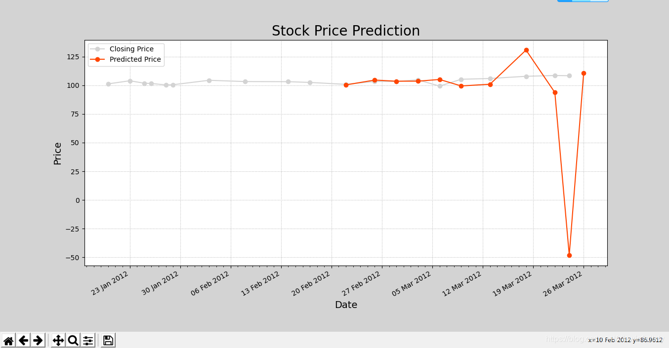
3、价格预测案例
import datetime as dt
import numpy as np
import matplotlib.pylab as mp
import matplotlib.dates as md
import pandas as pd
def dmy2ymd(dmy):
dmy = str(dmy, encoding='utf-8')
date = dt.datetime.strptime(dmy, '%d-%m-%Y').date()
ymd = date.strftime('%Y-%m-%d')
return ymd
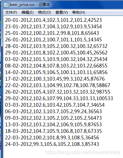
dates, closing_prices = np.loadtxt(
'0=数据源/beer_price.csv', delimiter=',',
usecols=(0, 4), unpack=True,
dtype=np.dtype('M8[D], f8'),
converters={0: dmy2ymd}
)
'''
收盘价格预测
'''
N = 5
pred_prices = np.zeros(closing_prices.size - 2*N + 1)
for i in range(pred_prices.size):
a = np.zeros((N, N))
for j in range(N):
a[j, ] = closing_prices[i+j: i+j+N]
b = closing_prices[i+N: i+N*2]
x = np.linalg.lstsq(a, b)[0]
pred_prices[i] = b.dot(x)
mp.figure('Stock Price Prediction', facecolor='lightgray')
mp.title('Stock Price Prediction', fontsize=20)
mp.xlabel('Date', fontsize=14)
mp.ylabel('Price', fontsize=14)
ax = mp.gca()
ax.xaxis.set_major_locator(
md.WeekdayLocator(byweekday=md.MO)
)
ax.xaxis.set_minor_locator(
md.DayLocator()
)
ax.xaxis.set_major_formatter(
md.DateFormatter('%d %b %Y')
)
mp.tick_params(labelsize=10)
mp.grid(linestyle=':')
dates = dates.astype(md.datetime.datetime)
mp.plot(dates, closing_prices, 'o-', c='lightgray', label="Closing Price")
dates = np.append(dates, dates[-1] + pd.tseries.offsets.BDay())
mp.plot(dates[N*2: ], pred_prices, 'o-', c='orangered', label='Predicted Price')
mp.legend()
mp.gcf().autofmt_xdate()
mp.show()
csv数据:

4、测试效果
二、线性拟合
1、基本概念
kx1 + b = y1
kx2 + b = y2
...
kxn + b = yn
/ x1 \    / k \    / y1 \
| x2  | x | b |  = | y2 |
|...  |   \   /    |... |
\ xn /             \ yn /

   a           x          b
2、numpy的对应函数
x = np.linalg.lstsq(a, b)
3、统计学知识
- 趋势点:设定的某几项数据的平均值(此处为最高价、最低价与收盘价的平均值)
- 压力点:趋势点+每天的幅度
- 支撑点:趋势点-每天的幅度
- 计算趋势线:日期乘斜率+截距
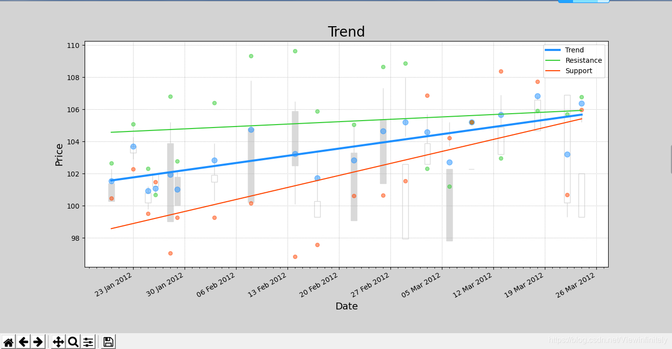
4、线性拟合趋势图案例
import datetime as dt
import numpy as np
import matplotlib.pylab as mp
import matplotlib.dates as md
def dmy2ymd(dmy):
dmy = str(dmy, encoding='utf-8')
date = dt.datetime.strptime(dmy, '%d-%m-%Y').date()
ymd = date.strftime('%Y-%m-%d')
return ymd
dates, opening_prices, highest_prices, lowest_prices, closing_prices = np.loadtxt(
'0=数据源/beer_price.csv', delimiter=',',
usecols=(0, 1, 2, 3, 4), unpack=True,
dtype='M8[D], f8, f8, f8, f8',
converters = {0:dmy2ymd}
)
trend_points = (highest_prices + lowest_prices + closing_prices) / 3
spreads = highest_prices - lowest_prices
resistance_points = trend_points + spreads
support_points = trend_points - spreads
days = dates.astype(int)
a = np.column_stack((days, np.ones_like(days)))
x1 = np.linalg.lstsq(a, trend_points)[0]
trend_line = days * x1[0] + x1[1]
x2 = np.linalg.lstsq(a, resistance_points)[0]
resistance_line = days * x2[0] + x2[1]
x3 = np.linalg.lstsq(a, support_points)[0]
support_line = days * x3[0] + x3[1]
mp.figure('Trend', facecolor='lightgray')
mp.title('Trend', fontsize=20)
mp.xlabel('Date', fontsize=14)
mp.ylabel('Price', fontsize=14)
ax = mp.gca()
ax.xaxis.set_major_locator(
md.WeekdayLocator(byweekday=md.MO)
)
ax.xaxis.set_minor_locator(
md.DayLocator()
)
ax.xaxis.set_major_formatter(md.DateFormatter('%d %b %Y'))
mp.tick_params(labelsize=10)
mp.grid(linestyle=':')
dates = dates.astype(md.datetime.datetime)
rise = closing_prices - opening_prices >= 0.01
fall = opening_prices - closing_prices >= 0.01
fc = np.zeros(dates.size, dtype='3f4')
ec = np.zeros(dates.size, dtype='3f4')
fc[rise], fc[fall] = (1, 1, 1), (0.85, 0.85, 0.85)
ec[rise], ec[fall] = (0.85, 0.85, 0.85), (0.85, 0.85, 0.85)
mp.bar(dates, highest_prices-lowest_prices, 0, lowest_prices, color=fc, edgecolor=ec)
mp.bar(dates, closing_prices-highest_prices, 0.8, opening_prices, color=fc, edgecolor=ec)
mp.scatter(dates, trend_points, c="dodgerblue", alpha=0.5, s=60, zorder=2)
mp.plot(dates, trend_line, c="dodgerblue", linewidth=3, label="Trend")
mp.scatter(dates, resistance_points, c="limegreen", alpha=0.5, s=30, zorder=2)
mp.plot(dates, resistance_line, c="limegreen", linewidth=1.5, label="Resistance")
mp.scatter(dates, support_points, c="orangered", alpha=0.5, s=30, zorder=2)
mp.plot(dates, support_line, c="orangered", linewidth=1.5, label="Support")
mp.gcf().autofmt_xdate()
mp.legend()
mp.show()
csv数据:
5、测试效果
本文内容由网友自发贡献,版权归原作者所有,本站不承担相应法律责任。如您发现有涉嫌抄袭侵权的内容,请联系:hwhale#tublm.com(使用前将#替换为@)