recognition mnist handwriting digits
download mnist and load data
MNIST can be downloaded in this website http://yann.lecun.com/exdb/mnist/.
After download data set, unzip it like this: tar -xzvf ‘****.gz’.
And there will two datasets and four files used by us in forward steps.
t10k-images.idx3-ubyte, t10k-labels.idx3-ubyte
train-images.idx3-ubyte, train-labels.idx3-ubyte
There are two functions provided to extract the data.
One is implemented in Python language.
The other is implemented in Matlab language.
function images = loadMNISTImages(filename)
%loadMNISTImages returns a [number of MNIST images]x28x28 matrix containing
%the raw MNIST images

fp = fopen(filename, 'rb');
assert(fp ~= -1, ['Could not open ', filename, '']);

magic = fread(fp, 1, 'int32', 0, 'ieee-be');
assert(magic == 2051, ['Bad magic number in ', filename, '']);

numImages = fread(fp, 1, 'int32', 0, 'ieee-be');
numRows = fread(fp, 1, 'int32', 0, 'ieee-be');
numCols = fread(fp, 1, 'int32', 0, 'ieee-be');

images = fread(fp, inf, 'unsigned char');
images = reshape(images, numCols, numRows, numImages);
images = permute(images,[2 1 3]);

fclose(fp);

% Reshape to #pixels x #examples
images = reshape(images, size(images, 1) * size(images, 2), size(images, 3));
% Convert to double and rescale to [0,1]
images = double(images) / 255;

end
function labels = loadMNISTLabels(filename)
%loadMNISTLabels returns a [number of MNIST images]x1 matrix containing
%the labels for the MNIST images

fp = fopen(filename, 'rb');
assert(fp ~= -1, ['Could not open ', filename, '']);

magic = fread(fp, 1, 'int32', 0, 'ieee-be');
assert(magic == 2049, ['Bad magic number in ', filename, '']);

numLabels = fread(fp, 1, 'int32', 0, 'ieee-be');

labels = fread(fp, inf, 'unsigned char');

assert(size(labels,1) == numLabels, 'Mismatch in label count');

fclose(fp);

end
The code above is provided by Prof. Andrew Ng.
The following code extracts data by Python.
Firstly, we should load the library we need.
# import libs we need
import numpy as np
import struct
import matplotlib.pyplot as plt
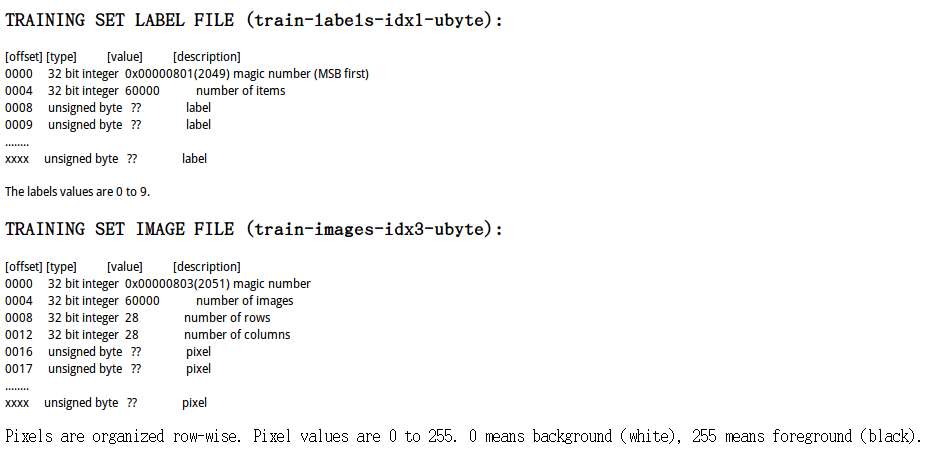
In LeCun’s blog, how the picture is saved has been illustrated in details.
# load data

def loadimg(imgfilename):
    with open(imgfilename, 'rb') as imgfile:
        datastr = imgfile.read()

    index = 0
    mgc_num, img_num, row_num, col_num = struct.unpack_from('>IIII', datastr, index)
    index += struct.calcsize('>IIII')

    image_array = np.zeros((img_num, row_num, col_num))
    for img_idx in xrange(img_num):
        img = struct.unpack_from('>784B', datastr, index)
        index += struct.calcsize('>784B')
        image_array[img_idx,:,:] = np.reshape(np.array(img), (28,28))
    image_array = image_array/255.0
    np.save(imgfilename[:6]+'image-py', image_array)
    return None

def loadlabel(labelfilename):
    with open(labelfilename, 'rb') as labelfile:
        datastr = labelfile.read()

    index = 0
    mgc_num, label_num = struct.unpack_from('>II', datastr, index)
    index += struct.calcsize('>II')

    label = struct.unpack_from('{}B'.format(label_num), datastr, index)
    index += struct.calcsize('{}B'.format(label_num))

    label_array = np.array(label)

    np.save(labelfilename[:5]+'label-py', label_array)
    return None
The two functions above are used to import data and save them as a python-fitting format (.npy).
loadimg('train-images.idx3-ubyte')
loadimg('t10k-images.idx3-ubyte')
loadlabel('train-labels.idx1-ubyte')
loadlabel('t10k-labels.idx1-ubyte')
Then it is easy to load data by numpy function.
train_image = np.load('train-image-py.npy')
train_label = np.load('trainlabel-py.npy')
test_image = np.load('t10k-iimage-py.npy')
test_label = np.load('t10k-label-py.npy')
What are the dimensions of our Array?
print(train_image.shape)
print(train_label.shape)
print(test_image.shape)
print(test_label.shape)
(60000, 28, 28)
(60000,)
(10000, 28, 28)
(10000,)
Loading one of the pictures, we can check whether the data is well saved. And then using matplotlib to display it, we get a digit picture.
# check data
%matplotlib inline
im = train_image[9,:,:]
im = 255*im
plt.imshow(im, cmap='gray')
plt.show()
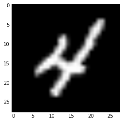
print(train_label[9])
4
im = test_image[17,:,:]
im = 255*im
plt.imshow(im, cmap='gray')
plt.show()
print(test_label[17])
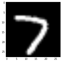
7
OK. Do we finish the data-preparation stage?
import tensorflow as tf
from six.moves import reduce
image_size = 28
num_labels = 10
num_channels = 1 # gray scale

reformat = lambda data,labels: (data.reshape((-1, image_size, image_size, 1)).astype(np.float32),(np.arange(num_labels) == labels[:,None]).astype(np.float32))
Sorry, we do not finish it yet.
For training networks, we have to change the dimensions of our data. What’s more, we will add one more variable for storing the label of each picture. Our label variable is in One-Hot encoding format. Thanks to tensorflow, it has provided reformatfunction to help us.
If you have doubts with convolution networks or One-Hot Encoding, you can find some detailed explanations in my former blogs: Convolution Networks,One-Hot Encoding
train_dataset, train_labels = reformat(train_image, train_label)
test_dataset, test_labels = reformat(test_image, test_label)
print('train_dataset size: ', train_dataset.shape)
print('train_labels size: ', train_labels.shape)
print('test_dataset size: ', test_dataset.shape)
print('test_labels size: ', test_labels.shape)
('train_dataset size: ', (60000, 28, 28, 1))
('train_labels size: ', (60000, 10))
('test_dataset size: ', (10000, 28, 28, 1))
('test_labels size: ', (10000, 10))
At this step, we have finished our preparation.
We have got train_dataset,train_labels,test_dataset,test_labels in right format.
accuracy = lambda pred, labels: (100.0 * np.sum(np.argmax(pred,1) == np.argmax(labels,1))/pred.shape[0] )
Function accuracy is used to compute the accuracy of our model.
Training and Testing
Our architecture of convolution network is based on the following picture.
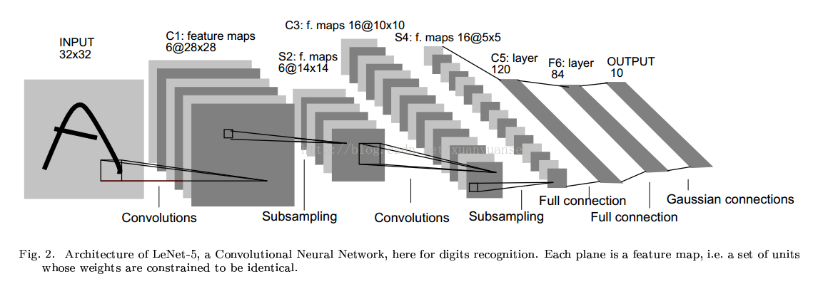
We define the architecture in the function model.
Due to the dimensions of our initial picture is (28,28), the first convolution in the picture is ignored by us.
The optimizer of gradient descend algorithm is used as:
tf.train.AdamOptimizer(learning_rate=0.001).minimize(loss) .
batch_size = 128

num_steps = 4501

graph = tf.Graph()
with graph.as_default():
    # Input data.
    tf_train_dataset = tf.placeholder(tf.float32, shape=(batch_size, image_size, image_size, num_channels)) # num_channels=1 grayscale
    tf_train_labels = tf.placeholder(tf.float32, shape=(batch_size, num_labels))
    tf_test_dataset = tf.constant(test_dataset)

        # Variables.

    filter1 = tf.Variable(tf.truncated_normal([1,1,1,6], stddev=0.1))
    biases1 = tf.Variable(tf.zeros([6]))

    filter2 = tf.Variable(tf.truncated_normal( [5,5,6,16], stddev=0.1))
    biases2 = tf.Variable(tf.constant(1.0, shape=[16]))

    filter3 = tf.Variable(tf.truncated_normal([5,5, 16, 120], stddev=0.1))
    biases3 = tf.Variable(tf.constant(1.0, shape=[120]))

    weights1 = tf.Variable(tf.truncated_normal([120, 84], stddev=0.1))
    w_biases1 = tf.Variable(tf.zeros([84]))
    weights2 = tf.Variable(tf.truncated_normal([84, 10], stddev=0.1))
    w_biases2 = tf.Variable(tf.zeros([10]))

    def model(data):
        # data (batch, 28, 28, 1)
        # filter1 (1, 1, 1, 6)
        conv = tf.nn.conv2d(data, filter1, [1,1,1,1], padding='SAME')
        conv = tf.nn.tanh(conv + biases1)
    # data reshaped to (batch, 28, 28, 1)
    # filter1 reshaped yo (1*1*1, 6)
    # conv shape (batch, 28, 28, 6)
    # sub-smapling
        conv = tf.nn.avg_pool(conv, [1,2,2,1], [1,2,2,1], padding='SAME')
    # conv shape(batch, 14, 14, 6)
    # filter2 shape(5, 5, 6, 16)
        conv = tf.nn.conv2d(conv, filter2, [1,1,1,1], padding='VALID')
    # conv reshaped to (batch, 10, 10, 5*5*6)
    # filter2 reshaped to (5*5*6, 16)
    # conv shape (batch, 10, 10, 16)
        conv = tf.nn.tanh(conv + biases2)
    # conv shape (batch, 10, 10, 16)
        conv = tf.nn.avg_pool(conv, [1,2,2,1], [1,2,2,1], padding='SAME')
    # conv shape (batch, 5,5 16)
    # filter3 shape (5,5, 16, 120)
        conv = tf.nn.conv2d(conv, filter3, [1,1,1,1], padding='VALID')
    # conv reshape( batch, 1, 1, 5*5*16)
    # filter3 reshape (5*5*16, 120)
    # conv = (batch, 1,1, 120)
        conv = tf.nn.tanh(conv + biases3)
        shape = conv.get_shape().as_list()
        reshape = tf.reshape(conv, (shape[0], reduce(lambda a,b:a*b, shape[1:])))
        hidden = tf.nn.relu(tf.matmul(reshape, weights1) + w_biases1)
        hidden = tf.nn.dropout(hidden, 0.8)
        logits = tf.matmul(hidden, weights2) + w_biases2
        return logits

     # Training computation.
    logits = model(tf_train_dataset)
    loss = tf.reduce_mean(tf.nn.softmax_cross_entropy_with_logits(logits, tf_train_labels))

        # Optimizer.
    optimizer = tf.train.AdamOptimizer(learning_rate=0.001).minimize(loss)

        # Predictions for the training, validation, and test data.
    train_prediction = tf.nn.softmax(logits)
    test_prediction = tf.nn.softmax(model(tf_test_dataset))


with tf.Session(graph=graph) as session:
    tf.initialize_all_variables().run()
    print('Initialized')
    for step in range(num_steps):
        offset = (step * batch_size) % (train_labels.shape[0] - batch_size)
        batch_data = train_dataset[offset:(offset + batch_size), :, :, :]
        batch_labels = train_labels[offset:(offset + batch_size), :]
        feed_dict = {tf_train_dataset : batch_data, tf_train_labels : batch_labels}
        _, l, predictions = session.run([optimizer, loss, train_prediction], feed_dict=feed_dict)
        if (step % 500 == 0):

            print('Minibatch loss at step %d: %f' % (step, l))

            print('Minibatch accuracy: %.1f%%' % accuracy(predictions, batch_labels))
    print('Test accuracy: %.1f%%' % accuracy(test_prediction.eval(), test_labels))
Initialized
Minibatch loss at step 0: 2.441036
Minibatch accuracy: 10.9%
Minibatch loss at step 500: 0.214182
Minibatch accuracy: 92.2%
Minibatch loss at step 1000: 0.086537
Minibatch accuracy: 97.7%
Minibatch loss at step 1500: 0.107810
Minibatch accuracy: 96.9%
Minibatch loss at step 2000: 0.088142
Minibatch accuracy: 97.7%
Minibatch loss at step 2500: 0.150886
Minibatch accuracy: 96.1%
Minibatch loss at step 3000: 0.088806
Minibatch accuracy: 98.4%
Minibatch loss at step 3500: 0.039191
Minibatch accuracy: 97.7%
Minibatch loss at step 4000: 0.018480
Minibatch accuracy: 99.2%
Minibatch loss at step 4500: 0.010719
Minibatch accuracy: 100.0%
Test accuracy: 98.2%
The accuracy rate is about 98%. However, that is not a good enough accuracy rate. There are several aspects of our model to be improved:
1. subsampling type: max pooling, average pooling, etc.
2. activate function: relu, tanh, etc.
3. initial value.