强化学习笔记-13 Policy Gradient Methods

2023-11-10

强化学习算法主要在于学习最优的决策，到目前为止，我们所讨论的决策选择都是通过价值预估函数来间接选择的。本节讨论的是通过一个参数化决策模型 $\pi(a|s,\theta )$ 来直接根据状态 $s$ 选择动作，而不是根据价值预估函数 $v(s|w)$ 来间接选择。

我们可以定义如下Policy Gradient更新策略，来求解参数化决策模型 $\pi(a|s,\theta )$ 的参数，其中 $J(\theta_t)$ 表示用于衡量决策模型优劣的损失函数。

$\theta_{t+1} = \theta_{t} + \partial_{\theta_{t}} J(\theta_t)$

1. Policy Approximation and its Advantages

对于参数化决策模型 $\pi(a|s,\theta )$ 存在两种建模方式：生成式或判别式。

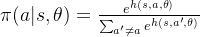
当动作空间是离散且较小时，可以采用判别式模型 $h(s,a,\theta )$ ，表示状态-动作对 $s,a$ 的优劣得分，此时 $\pi(a|s,\theta )$ 可以表示为下式，这种通过softmax求得选择动作概率，兼顾了ε-greedy动作探索的功能。另一方面在很多情况下随机动作也是最优的，softmax方式具备这种特性。

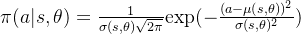
$\pi(a|s,\theta )=\frac{e^{h(s,a,\theta)}}{\sum_{a'\neq a}e^{h(s,a',\theta)}}$

当动作空间是连续时，生成式模型是一个比较好选择，一种简单方式是将决策动作分布 $\pi(a|s,\theta )$ 建模为一个高斯分布，由于动作分布方差的存在，因此也兼顾了动作探索的特性。

$\pi(a|s,\theta)=\frac{1}{\sigma(s,\theta)\sqrt{2\pi}}\text{exp}(-\frac{(a-\mu(s,\theta))^2}{\sigma(s,\theta)^2})$

2. The Policy Gradient Theorem

接下来关键在于如何找到一个衡量决策模型优劣的损失函数 $J(\theta_t)$ 。直观上理解，在最优决策下，各状态价值应该也是最优的，因此可以定义：

$J(\theta)=\sum_s \mu(s) \sum_a \pi(a|s,\theta) Q(s,a)$

此时有

$\partial J(\theta)\\=\sum_s \mu(s) \sum_a Q(s,a) \partial_{\theta}\pi(a|s,\theta) \\=\sum_s \mu(s) \sum_a Q(s,a)\pi(a|s,\theta) \frac{\partial_{\theta}\pi(a|s,\theta)}{\pi(a|s,\theta) }\\=E[G(s,a)\frac{\partial_{\theta}\pi(a|s,\theta)}{\pi(a|s,\theta)}]$

可以定义如下SGD更新参数式子：

$\theta_{t+1}=\theta_{t} + \beta G_t(s,a) \frac{\partial_{\theta}\pi(a|s,\theta_t)}{\pi(a|s,\theta_t)}$

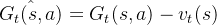
根据上式，同MC结合的Policy Gradient Methods：

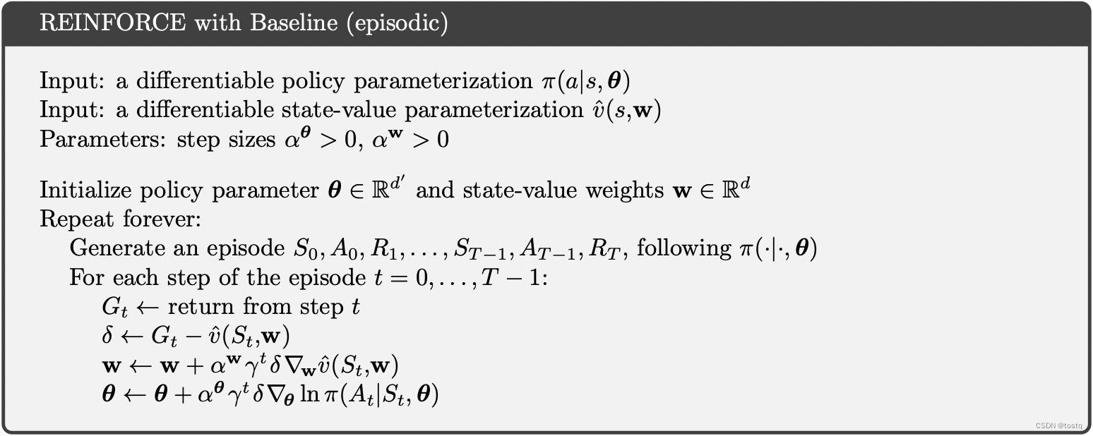
3. Baseline

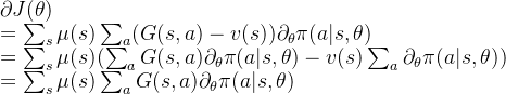
因为参数化决策模型中参数 $\theta$ 在不同 $s,a$ 下会同步更新，因此某些状态 $s$ 下其累积收益 $G$ 远大于其他状态，而决策模型是根据状态来选择动作，所以不同状态 $s$ 下其累积收益 $G$ 不同，会引入偏差，这个偏差会影响模型的影响。

因此可以对累积收益 $G$ 减去状态带来的偏差，即

$\hat{G_t(s,a)}=G_t(s,a)-v_t(s)$

此时参数更新可以变为：

$\theta_{t+1}=\theta_{t} + \beta (G_t(s,a) - v_t(s))\frac{\partial_{\theta}\pi(a|s,\theta_t)}{\pi(a|s,\theta_t)}$

另外也可以看出虽然减去状态带来的偏差因子，原来同损失函数 $J(\theta_t)$ 也是等价的。

$\partial J(\theta)\\=\sum_s \mu(s) \sum_a (G(s,a) -v(s))\partial_{\theta}\pi(a|s,\theta)\\=\sum_s \mu(s) (\sum_a G(s,a)\partial_{\theta}\pi(a|s,\theta) - v(s)\sum_a \partial_{\theta}\pi(a|s,\theta))\\ =\sum_s \mu(s) \sum_a G(s,a)\partial_{\theta}\pi(a|s,\theta)$

4. Actor–Critic Methods

$\theta_{t+1}=\theta_{t} + \beta (R_{t+1} + \gamma v(s_{t+1}|w_t) - v_t(s|w_t))\frac{\partial_{\theta_t}\pi(a|s,\theta_t)}{\pi(a|s,\theta_t)} \\ w_{t+1}=w_t + \alpha (R_{t+1} + \gamma v(s_{t+1}|w_t) - v_t(s|w_t))\partial_{w_t} v(s|w_t)$

本文内容由网友自发贡献，版权归原作者所有，本站不承担相应法律责任。如您发现有涉嫌抄袭侵权的内容，请联系:hwhale#tublm.com(使用前将#替换为@)