具体来说,图像感知压缩模型的训练过程如下:给定图像
x
∈
R
H
×
W
×
3
x\in \mathbb{R}^{H\times W\times 3}
x∈RH×W×3,我们先利用一个编码器
ε
\varepsilon
ε来将图像从原图编码到潜在表示空间(即提取图像的特征)
z
=
ε
(
x
)
z=\varepsilon(x)
z=ε(x),其中
z
∈
R
h
×
w
×
c
z\in \mathbb{R}^{h\times w\times c}
z∈Rh×w×c。然后,用解码器从潜在表示空间重建图片
x
~
=
D
(
z
)
=
D
(
ε
(
x
)
)
\widetilde{x}=\mathcal{D}(z)=\mathcal{D}(\varepsilon(x))
x=D(z)=D(ε(x))。训练的目标是使
x
=
x
~
x=\widetilde{x}
x=x。
(2) 隐扩散模型(Latent Diffusion Models)
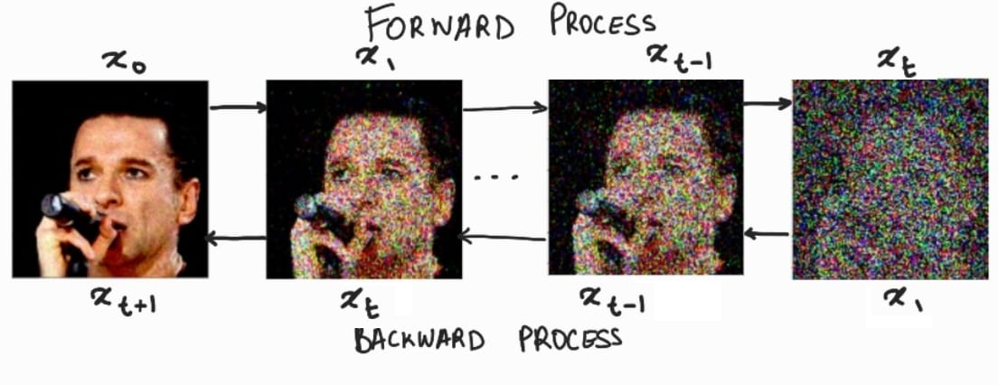
扩散模型(DM)从本质上来说,是一个基于马尔科夫过程的去噪器。其反向去噪过程的目标是根据输入的图像
x
t
x_t
xt去预测一个对应去噪后的图像
x
t
+
1
x_{t+1}
xt+1,即
x
t
+
1
=
ϵ
t
(
x
t
,
t
)
,
t
=
1
,
.
.
.
,
T
x_{t+1}=\epsilon_t(x_t,t),\ t=1,...,T
xt+1=ϵt(xt,t),t=1,...,T。相应的目标函数可以写成如下形式:
L
D
M
=
E
x
,
ϵ
∼
N
(
0
,
1
)
,
t
=
[
∣
∣
ϵ
−
ϵ
θ
(
x
t
,
t
)
∣
∣
2
2
]
L_{DM}=\mathbb{E}_{x,\epsilon\sim\mathcal{N(0,1),t}}=[||\epsilon-\epsilon_\theta(x_t,t)||_{2}^{2}]
LDM=Ex,ϵ∼N(0,1),t=[∣∣ϵ−ϵθ(xt,t)∣∣22]这里默认噪声的分布是高斯分布
N
(
0
,
1
)
\mathcal{N(0,1)}
N(0,1),这是因为高斯分布可以应用重参数化技巧简化计算;此处的
x
x
x指的是原图。
而在潜在扩散模型中(LDM),引入了预训练的感知压缩模型,它包括一个编码器
ε
\varepsilon
ε 和一个解码器
D
\mathcal{D}
D。这样在训练时就可以利用编码器得到
z
t
=
ε
(
x
t
)
z_t=\varepsilon(x_t)
zt=ε(xt),从而让模型在潜在表示空间中学习,相应的目标函数可以写成如下形式:
L
L
D
M
=
E
ε
(
x
)
,
ϵ
∼
N
(
0
,
1
)
,
t
=
[
∣
∣
ϵ
−
ϵ
θ
(
z
t
,
t
)
∣
∣
2
2
]
L_{LDM}=\mathbb{E}_{\varepsilon(x),\epsilon\sim\mathcal{N(0,1),t}}=[||\epsilon-\epsilon_\theta(z_t,t)||_{2}^{2}]
LLDM=Eε(x),ϵ∼N(0,1),t=[∣∣ϵ−ϵθ(zt,t)∣∣22]
(3) 条件机制(Conditioning Mechanisms) 条件机制,指的是通过输入某些参数来控制图像的生成结果。这主要是通过拓展得到一个条件时序去噪自编码器(Conditional Denoising Autoencoder,CDA)
ϵ
θ
(
z
t
,
t
,
y
)
\epsilon_\theta(z_t,t,y)
ϵθ(zt,t,y)来实现的,这样一来我们就可通过输入参数
y
y
y 来控制图像生成的过程。
具体来说,论文通过在UNet主干网络上增加cross-attention机制来实现CDA,选用UNet网络是因为实践中Diffusion在UNet网络上效果最好。为了能够从多个不同的模态预处理参数
y
y
y,论文引入了一个领域专用编码器(Domain Specific Encoder)
τ
θ
\tau_\theta
τθ,它将
y
y
y映射为一个中间表示
τ
θ
(
y
)
∈
R
M
×
d
r
\tau_\theta(y)\in\mathbb{R}^{M\times d_r}
τθ(y)∈RM×dr,这样我们就可以很方便的将
y
y
y设置为各种模态的条件(文本、类别等等)。最终模型就可以通过一个cross-attention层映射将控制信息融入到UNet的中间层,cross-attention层的实现如下:
A
t
t
e
n
t
i
o
n
(
Q
,
K
,
V
)
=
s
o
f
t
m
a
x
(
Q
K
⊤
d
)
⋅
V
Attention(Q,K,V)=softmax(\frac{QK^\top}{\sqrt{d}})\cdot V
Attention(Q,K,V)=softmax(dQK⊤)⋅V
Q
=
W
Q
(
i
)
⋅
φ
i
(
z
t
)
,
K
=
W
K
(
i
)
⋅
τ
θ
(
y
)
,
V
=
W
V
(
i
)
⋅
τ
θ
(
y
)
Q=W_{Q}^{(i)}\cdot \varphi_i(z_t),\quad K=W_{K}^{(i)}\cdot \tau_\theta(y),\quad V=W_{V}^{(i)}\cdot \tau_\theta(y)
Q=WQ(i)⋅φi(zt),K=WK(i)⋅τθ(y),V=WV(i)⋅τθ(y)其中
φ
i
(
z
t
)
∈
R
N
×
d
ϵ
i
\varphi_i(z_t)\in \mathbb{R}^{N\times d_{\epsilon}^{i}}
φi(zt)∈RN×dϵi 是UNet的一个中间表征;
W
Q
(
i
)
W_{Q}^{(i)}
WQ(i)、
W
K
(
i
)
W_{K}^{(i)}
WK(i)和
W
V
(
i
)
W_{V}^{(i)}
WV(i)分别是三个权重矩阵。此时,带有条件机制的隐扩散模型的目标函数可以写成如下形式:
L
L
D
M
=
E
ε
(
x
)
,
y
,
ϵ
∼
N
(
0
,
1
)
,
t
=
[
∣
∣
ϵ
−
ϵ
θ
(
z
t
,
t
,
τ
θ
(
y
)
)
∣
∣
2
2
]
L_{LDM}=\mathbb{E}_{\varepsilon(x),\ y,\ \epsilon\sim\mathcal{N(0,1),\ t}}=[||\epsilon-\epsilon_\theta(z_t,\ t,\ \tau_\theta(y))||_{2}^{2}]
LLDM=Eε(x),y,ϵ∼N(0,1),t=[∣∣ϵ−ϵθ(zt,t,τθ(y))∣∣22]
# move Model to the GPU
torch.cuda.empty_cache()
pipe = pipe.to("cuda")# V1 Max-H:512,Max-W:512# V2 Max-H:768,Max-W:768print(datetime.datetime.now())# 提示词,一句话或者多句话
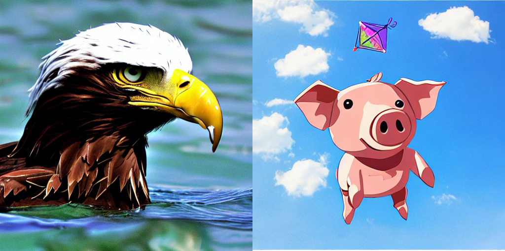
prompts =["An eagle flying in the water","A pig kite flying in the sky",]
generated_images = pipe(
prompt=prompts,
height=512,# 生成图像的高度
width=512,# 生成图像的宽度
num_images_per_prompt=1# 每个提示词生成多少个图像).images # image here is in [PIL format](https://pillow.readthedocs.io/en/stable/)print(f"Prompts: {prompts}\n")print(datetime.datetime.now())for image in generated_images:
display(image)
# 提交json数据,接收生成的图像数据
response = predictor[SD_MODEL].predict(data={"prompt":["An eagle flying in the water",# "A pig kite flying in the sky",],"height":512,"width":512,"num_images_per_prompt":1})# 解码生成的图像
decoded_images =[decode_base64_image(image)for image in response["generated_images"]]#visualize generationfor image in decoded_images:
display(image)
我们构建的推理脚本将模型的功能解耦成两个函数,实际上就是读取模型以及读取超参数和prompts:
defmodel_fn(model_dir):# Load stable diffusion and move it to the GPU
pipe = StableDiffusionPipeline.from_pretrained(model_dir, torch_dtype=torch.float16)
pipe = pipe.to("cuda")return pipe
defpredict_fn(data, pipe):# get prompt & parameters
prompt = data.pop("prompt","")# set valid HP for stable diffusion
height = data.pop("height",512)
width = data.pop("width",512)
num_inference_steps = data.pop("num_inference_steps",50)
guidance_scale = data.pop("guidance_scale",7.5)
num_images_per_prompt = data.pop("num_images_per_prompt",1)# run generation with parameters
generated_images = pipe(
prompt=prompt,
height=height,
width=width,
num_inference_steps=num_inference_steps,
guidance_scale=guidance_scale,
num_images_per_prompt=num_images_per_prompt,)["images"]# create response
encoded_images =[]for image in generated_images:
buffered = BytesIO()
image.save(buffered,format="JPEG")
encoded_images.append(base64.b64encode(buffered.getvalue()).decode())# create responsereturn{"generated_images": encoded_images}
from sagemaker.s3 import S3Uploader
sd_model_uri=S3Uploader.upload(local_path=f"{SD_MODEL}.tar.gz", desired_s3_uri=f"s3://{sess.default_bucket()}/stable-diffusion")#init variables
huggingface_model ={}
predictor ={}from sagemaker.huggingface.model import HuggingFaceModel
# create Hugging Face Model Class
huggingface_model[SD_MODEL]= HuggingFaceModel(
model_data=sd_model_uri,# path to your model and script
role=role,# iam role with permissions to create an Endpoint
transformers_version="4.17",# transformers version used
pytorch_version="1.10",# pytorch version used
py_version='py38',# python version used)# deploy the endpoint endpoint, Estimated time to spend 5min(V1), 8min(V2)
predictor[SD_MODEL]= huggingface_model[SD_MODEL].deploy(
initial_instance_count=1,
instance_type="ml.g4dn.xlarge",
endpoint_name=f"{SD_MODEL}-endpoint")