02_End-to-End Machine Learning Project
https://blog.csdn.net/Linli522362242/article/details/103387527
Here are the main steps you will go through:
1. Look at the big picture.
-
Frame the Problem
-
What is the business objective, How does the company expect to use and benefit from the model
- Your boss answers that your model’s output (a prediction of a district’s median housing price
-
What the current solution looks like (if any). It will often give you a reference performance, as well as insights on how to solve the problem.
- Your boss answers that the district housing prices are currently estimated manually by experts
-
Frame the problem: is it supervised, unsupervised, or Reinforcement Learning? Is it a classification task, a regression task, or something else? Should you use batch learning or online learning techniques?
- it is clearly a typical supervised learning task since you are given labeled training examples (each instance comes with the expected output, i.e., the district’s median housing price). Moreover, it is also a typical regression task, since you are asked to predict a value. More specifically, this is a multivariate regression problem since the system will use multiple features to make a prediction (it will use the district’s population, the median income, etc.). In the first chapter, you predicted life satisfaction based on just one feature, the GDP per capita, so it was a univariate regression problem. Finally, there is no continuous flow of data coming in the system, there is no particular need to adjust to changing data rapidly, and the data is small enough to fit in memory, so plain batch learning should do just fine.
-
Select a Performance Measure
- A typical performance measure for regression problems is the Root Mean Square Error (RMSE corresponds to the Euclidian norm)
-
 The higher the norm index(k), the more it focuses on large values and neglects small ones. This is why the RMSE is more sensitive to outliers than the MAE(Mean Absolute Error --Manhattan norm). But when outliers are exponentially rare (like in a bell-shaped curve), the RMSE performs very well and is generally preferred.
- the “68-95-99.7” rule applies: about 68% of the values fall within 1σ of the mean,
95% within 2σ, and
99.7% within 3σ.
-
Check the Assumptions
- your system outputs are going to be fed into a downstream Machine Learning system, and we assume that these prices are going to be used as such(regression task). But what if the downstream system actually converts the prices into categories (e.g., “cheap,” “medium,” or “expensive”) and then uses those categories instead of the prices themselves? In this case, getting the price perfectly right is not important at all; your system just needs to get the category right. If that’s so, then the problem should have been framed as a classification task, not a regression task. You don’t want to find this out after working on a regression system for months.
2. Get the data.
-
Create the Workspace
- create a workspace directory for your Machine Learning code

- and datasets.

- Download the Data
-
Take a Quick Look at the Data Structure
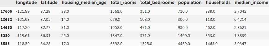
- housing.head()
- housing.info (total number of rows, and each attribute’s type and number of non-null values~~the amount of missing value) ; housing["ocean_proximity"].value_counts()
- housing.describe() method shows a summary of the numerical attributes
- housing.hist() : Notice a few things
-
Create a Test Set (create a test set(typically 20% of the dataset), put it aside, and never look at it)
-
purely random sampling
- train_set, test_set = train_test_split(housing, test_size=0.2, random_state=42)
-
stratified sampling
- Suppose you chatted with experts who told you that the median income is a very important attribute to predict median housing prices. You may want to ensure that the test set is representative of the various categories of incomes in the whole dataset. Since the median income is a continuous numerical attribute, you first need to create an income category attribute. Let’s look at the median income histogram more closely
-
housing['median_income'].hist() #a continuous numerical attribute --5 Categries
-
housing['income_cat'] = pd.cut(housing['median_income'],
                               bins=[0., 1.5, 3.0, 4.5, 6., np.inf],
                               labels=[1,2,3,4,5]
                              )
housing['income_cat'].value_counts()
housing["income_cat"].hist()
- The following code creates an income category attribute by dividing the median income by 1.5 (to limit the number of income categories), and rounding up using ceil (to have discrete categories), and then merging all the categories greater than 5 into category 5:
housing["income_cat"] = np.ceil(housing["median_income"] / 1.5)
housing["income_cat"].where(housing["income_cat"] < 5, 5.0, inplace=True)
-
Now you are ready to do stratified sampling based on the income category. For this you can use Scikit-Learn’s StratifiedShuffleSplit class:
from sklearn.model_selection import StratifiedShuffleSplit

                              #n_splits: n groups of train/test pair
split = StratifiedShuffleSplit(n_splits=1, test_size=0.2, random_state=42) #one group of train/test pair
for train_index, test_index in split.split(housing, housing['income_cat']):
    strat_train_set = housing.loc[train_index]
    strat_test_set = housing.loc[test_index]
looking at the income category proportions in the full housing dataset:
housing["income_cat"].value_counts() / len(housing)
you can measure the income category proportions in the test set
strat_test_set["income_cat"].value_counts()/len(strat_test_set)
Sampling bias comparison of stratified versus purely random sampling
3. Now you should remove the income_cat attribute so the data is back to its original state:
for set in (strat_train_set, strat_test_set):
set.drop(["income_cat"], axis=1, inplace=True)
3. Discover and visualize the data to gain insights.(plot)
-
First, make sure you have put the test set aside and you are only exploring the training set. Also, if the training set is very large, you may want to sample an exploration set, to make manipulations easy and fast. In our case, the set is quite small so you can just work directly on the full set. Let’s create a copy so you can play with it without harming the training set:
housing = strat_train_set.copy() #df.copy(deep=True) #https://blog.csdn.net/weixin_37275456/article/details/83033528
#https://blog.csdn.net/u010712012/article/details/79754132
-
housing.plot(kind="scatter", x="longitude", y="latitude", alpha=0.1,
             title="A better visualization highlighting high-density areas")
-
Looking for Correlations¶:Since the dataset is not too large, you can easily compute the standard correlation coefficient (also called Pearson’s r) between every pair of attributes using the corr() method:
corr_matrix = housing.corr()
corr_matrix["median_house_value"].sort_values(ascending=False)
The most promising最有希望的 attribute to predict the median house value is the median income
Since there are now 11 numerical attributes, you would get 11^2 = 121 plots, which would not fit on a page, so let’s just focus on a few promising attributes that seem most correlated with the median housing value (Figure):
from pandas.plotting import scatter_matrix
attributes = ["median_house_value", "median_income", "total_rooms", "housing_median_age"]
scatter_matrix(housing[attributes], figsize=(12,8))
plt.show()
4. Experimenting with Attribute Combinations:The new bedrooms_per_room attribute is much more correlated with the median house value than the total number of rooms or bedrooms
4. Prepare the data for Machine Learning algorithms.
- Instead of just doing this manually, you should write functions to do that, for several good reasons:
• This will allow you to reproduce these transformations easily on any dataset (e.g., the next time you get a fresh dataset).
• You will gradually build a library of transformation functions that you can reuse in future projects.
• You can use these functions in your live system to transform the new data before feeding it to your algorithms.
• This will make it possible for you to easily try various transformations and see which combination of transformations works best.
-
housing = strat_train_set.drop('median_house_value', axis=1)  #return a dataframe without the dropped item
housing_label = strat_train_set["median_house_value"].copy()
housing.keys()
- Data Cleaning
- Most Machine Learning algorithms cannot work with missing features, so let’s create a few functions to take care of them. You noticed earlier that the total_bedrooms attribute has some missing values, so let’s fix this. You have three options:
• Get rid of the corresponding districts.
• Get rid of the whole attribute.
• Set the values to some value (zero, the mean, the median, etc.).
You can accomplish these easily using DataFrame’s dropna(), drop(), and fillna()
methods:
housing.dropna(subset=["total_bedrooms"]) # option 1
housing.drop("total_bedrooms", axis=1) # option 2
median = housing["total_bedrooms"].median()# option 3
housing["total_bedrooms"].fillna(median) # option 3
- Handling Text and Categorical Attributes
-
from sklearn.base import BaseEstimator, TransformerMixin
from sklearn.utils import check_array
from sklearn.preprocessing import LabelEncoder
from scipy import sparse

class CategoricalEncoder(BaseEstimator, TransformerMixin):
    def __init__(self, encoding='onehot', categories='auto', dtype=np.float64, handle_unknown='error'):
        self.encoding = encoding
        self.categories = categories
        self.dtype = dtype
        self.handle_unknown = handle_unknown

    def fit(self, X, y=None):
        """Fit the CategoricalEncoder to X.
        Parameters
        ----------
        X : array-like, shape [n_samples, n_feature]
        The data to determine the categories of each feature.
        Returns
        -------
        self
        """
        if self.encoding not in ['onehot', 'onehot-dense', 'ordinal']:
            template = ("encoding should be either 'onehot', 'onehot-dense' or 'ordinal', got %s")
            raise ValueError(template % self.handle_unknown)

        if self.handle_unknown not in ['error', 'ignore']:
            template = ("handle_unknown should be either 'error' or 'ignore', got %s")
            raise ValueError(template % self.handle_unknown)

        if self.encoding == 'ordinal' and self.handle_unknown == 'ignore':
            raise ValueError("handle_unknown='ignore' is not supported for encoding='ordinal'")

        #check_array: By default, the input(here is X) is converted to an at least 2D numpy array.
        #If the dtype of the array is object, attempt converting to float, raising on failure.
        #csc_matrix: https://docs.scipy.org/doc/scipy/reference/generated/scipy.sparse.csc_matrix.html
        X = check_array(X, dtype=np.object, accept_sparse='csc', copy=True)
        n_samples, n_features = X.shape   #(16512, 1)

        #the prefix underscore: private variable,
        #the trailing underscore is used by convention to avoid naming conflicts
        self._label_encoders_ = [LabelEncoder() for _ in range(n_features)]    #[LabelEncoder, ...]
        for i in range(n_features):
            le = self._label_encoders_[i]
            Xi = X[:, i]
            if self.categories == 'auto':
                le.fit(Xi)
            else:
                #np.in1d(ar1,ar2): Returns a boolean array the same length as ar1 that
                #is True where an element of ar1 is in ar2
                #and False otherwise.
                valid_mask = np.in1d(Xi, self.categories[i])
                if not np.all(valid_mask):
                    if self.handle_unknown == 'error':
                        diff = np.unique(Xi[~valid_mask])
                        msg = ("Found unknown categories {0} in column {1} during fit".format(diff, i))
                        raise ValueError(msg)
                le.classes_ = np.array(np.sort(self.categories[i]))
        #for examples,here is ['<1H OCEAN' 'INLAND' 'ISLAND' 'NEAR BAY' 'NEAR OCEAN']
        #encoder.classes_
        self.categories_ = [le.classes_ for le in self._label_encoders_]
        return self

    def transform(self, X):
        """Transform X using one-hot encoding.
        Parameters
        ----------
        X : array-like, shape [n_samples, n_features]
        The data to encode.
        Returns
        -------
        X_out : sparse matrix or a 2-d array
        Transformed input.
        """
        #check_array: By default, the input(here is X) is converted to an at least 2D numpy array.
        #If the dtype of the array is object, attempt converting to float, raising on failure.
        #csc_matrix: https://docs.scipy.org/doc/scipy/reference/generated/scipy.sparse.csc_matrix.html
        X = check_array(X, accept_sparse='csc', dtype=np.object, copy=True)
        n_samples, n_features = X.shape
        X_int = np.zeros_like(X, dtype=np.int)
        X_mask = np.ones_like(X, dtype=np.bool) #dtype:Overrides the data type of the result
                                                #conver the 1s to all True

        for i in range(n_features):
            #Returns a boolean array the same length as ar1 that is True where an element of ar1 is in ar2
            #and False otherwise.
            valid_mask = np.in1d(X[:, i], self.categories_[i]) #[ True  True  True ...  True  True  True]

            if not np.all(valid_mask):
                if self.handle_unknown == 'error':
                    diff = np.unique(X[~valid_mask, i])
                    msg = ("Found unknown categories {0} in column {1} during transform".format(diff, i))
                    raise ValueError(msg)
                else:
                    # Set the problematic rows to an acceptable value and
                    # continue `The rows are marked `X_mask` and will be
                    # removed later.
                    X_mask[:, i] = valid_mask
                    X[:, i][~valid_mask] = self.categories_[i][0]
            X_int[:, i] = self._label_encoders_[i].transform(X[:, i])  #[0 0 4 ... 1 0 3]  here only one column #len(row_indices)

            if self.encoding == 'ordinal':
                return X_int.astype(self.dtype, copy=False)
            mask = X_mask.ravel() #[ True  True  True ...  True  True  True]
           #self.categories_: [array(['<1H OCEAN', 'INLAND', 'ISLAND', 'NEAR BAY', 'NEAR OCEAN'], dtype=object)]
           #cats.shape[0]: 5
            n_values = [cats.shape[0] for cats in self.categories_] #[[5]]
            n_values = np.array([0] + n_values)   #np.array( [[0] [5]] )
            indices = np.cumsum(n_values)   #[0 5]  #start with 0, size=5 columns


            #X_int:  2D numpy array, here only one column
            #indices[:-1] : [0]
            #X_int + indices[:-1]: #matrix plus#[ [0 0 4 ... 1 0 3]^T ]
            column_indices = (X_int + indices[:-1]).ravel()[mask]    #extraction: [0 0 4 ... 1 0 3]
            row_indices = np.repeat(np.arange(n_samples, dtype=np.int32),n_features)[mask]
            data = np.ones(n_samples * n_features)[mask]
            #csc_matrix: https://docs.scipy.org/doc/scipy/reference/generated/scipy.sparse.csc_matrix.html

                                                                 #position  #len(row_indices)==len(column_indices)
            out = sparse.csc_matrix((data, (row_indices, column_indices)),
                                     shape=(n_samples, indices[-1]),  #(16512,5)
                                     dtype=self.dtype
                                   ).tocsr()
            if self.encoding == 'onehot-dense':
                return out.toarray()
            else:
                return out

        Parameters
        ----------
        X : array-like, shape [n_samples, n_feature]
        The data to determine the categories of each feature.
        Returns
        -------
        self
        """
        if self.encoding not in ['onehot', 'onehot-dense', 'ordinal']:
            template = ("encoding should be either 'onehot', 'onehot-dense' or 'ordinal', got %s")
            raise ValueError(template % self.handle_unknown)

        if self.handle_unknown not in ['error', 'ignore']:
            template = ("handle_unknown should be either 'error' or 'ignore', got %s")
            raise ValueError(template % self.handle_unknown)

        if self.encoding == 'ordinal' and self.handle_unknown == 'ignore':
            raise ValueError("handle_unknown='ignore' is not supported for encoding='ordinal'")
        X = check_array(X, dtype=np.object, accept_sparse='csc', copy=True)
        n_samples, n_features = X.shape

        self._label_encoders_ = [LabelEncoder() for _ in range(n_features)]
        for i in range(n_features):
            le = self._label_encoders_[i]
            Xi = X[:, i]
            if self.categories == 'auto':
                le.fit(Xi)
            else:
                valid_mask = np.in1d(Xi, self.categories[i])
                if not np.all(valid_mask):
                    if self.handle_unknown == 'error':
                        diff = np.unique(Xi[~valid_mask])
                        msg = ("Found unknown categories {0} in column {1} during fit".format(diff, i))
                        raise ValueError(msg)
                le.classes_ = np.array(np.sort(self.categories[i]))
        self.categories_ = [le.classes_ for le in self._label_encoders_]
        return self

    def transform(self, X):
        """Transform X using one-hot encoding.
        Parameters
        ----------
        X : array-like, shape [n_samples, n_features]
        The data to encode.
        Returns
        -------
        X_out : sparse matrix or a 2-d array
        Transformed input.
        """
        X = check_array(X, accept_sparse='csc', dtype=np.object, copy=True)
        n_samples, n_features = X.shape
        X_int = np.zeros_like(X, dtype=np.int)
        X_mask = np.ones_like(X, dtype=np.bool)

        for i in range(n_features):
            valid_mask = np.in1d(X[:, i], self.categories_[i])

            if not np.all(valid_mask):
                if self.handle_unknown == 'error':
                    diff = np.unique(X[~valid_mask, i])
                    msg = ("Found unknown categories {0} in column {1} during transform".format(diff, i))
                    raise ValueError(msg)
                else:
                    # Set the problematic rows to an acceptable value and
                    # continue `The rows are marked `X_mask` and will be
                    # removed later.
                    X_mask[:, i] = valid_mask
                    X[:, i][~valid_mask] = self.categories_[i][0]
            X_int[:, i] = self._label_encoders_[i].transform(X[:, i])

            if self.encoding == 'ordinal':
                return X_int.astype(self.dtype, copy=False)
            mask = X_mask.ravel()
            n_values = [cats.shape[0] for cats in self.categories_]
            n_values = np.array([0] + n_values)
            indices = np.cumsum(n_values)

            column_indices = (X_int + indices[:-1]).ravel()[mask]
            row_indices = np.repeat(np.arange(n_samples, dtype=np.int32),n_features)[mask]
            data = np.ones(n_samples * n_features)[mask]

            out = sparse.csc_matrix((data, (row_indices, column_indices)),
                                    shape=(n_samples, indices[-1]),
                                    dtype=self.dtype).tocsr()
            if self.encoding == 'onehot-dense':
                return out.toarray()
            else:
                return out

#from sklearn.preprocessing import CategoricalEncoder # in future versions of Scikit-Learn
cat_encoder = CategoricalEncoder()
housing_cat_reshaped = housing_cat.values.reshape(-1,1)
- Custom Transformers
- Feature Scaling:
-
min-max scaling(called normalization) : We do this by subtracting
the min value and dividing by the max minus the min.
-
standardization: first it subtracts the mean value (so standardized
values always have a zero mean), and then it divides by the variance so that the resulting
distribution has unit variance.
- Transformation Pipelines
-
from sklearn.pipeline import FeatureUnion #Sckit-learn <0.20
from sklearn.pipeline import Pipeline
from sklearn.preprocessing import StandardScaler

housing_num = housing.drop('ocean_proximity', axis=1)#return a dataframe without the dropped column
num_attribs = list(housing_num)
cat_attribs = ["ocean_proximity"]

num_pipeline=Pipeline([
    ('selector', DataFrameSelector(num_attribs)),
    ('imputer', Imputer(strategy='median')),
    ('attribs_adder', CombinedAttributesAdder()),
    ('std_scaler', StandardScaler()),
])

cat_pipeline = Pipeline([
    ('selector', DataFrameSelector(cat_attribs)),
    ('label_binarizer', CategoricalEncoder(encoding="onehot-dense"))
])

full_pipeline = FeatureUnion(n_jobs=1, #default 1
                            transformer_list=[('num_pipeline', num_pipeline),
                                              ('cat_pipeline', cat_pipeline),
                                             ]
                            )

housing_prepared = full_pipeline.fit_transform(housing)
5. Select a model and train it.
6. Fine-tune your model.
7. Present your solution.
8. Launch, monitor, and maintain your system
#################################TypeError: fit_transform() takes 2 positional arguments but 3 were given
from sklearn.pipeline import FeatureUnion #Sckit-learn <0.20
from sklearn.pipeline import Pipeline
from sklearn.preprocessing import StandardScaler
housing_num = housing.drop('ocean_proximity', axis=1)#return a dataframe without the dropped column
num_attribs = list(housing_num)
cat_attribs = ["ocean_proximity"]
num_pipeline=Pipeline([
('selector', DataFrameSelector(num_attribs)),
('imputer', Imputer(strategy='median')),
('attribs_adder', CombinedAttributesAdder()),
('std_scaler', StandardScaler()),
])
cat_pipeline = Pipeline([
('selector', DataFrameSelector(cat_attribs)), #
('label_binarizer',LabelBinarizer()) #CategoricalEncoder(encoding="onehot-dense")
])
full_pipeline = FeatureUnion(n_jobs=1, #default 1
transformer_list=[('num_pipeline', num_pipeline),
('cat_pipeline', cat_pipeline),
]
)
housing_prepared = full_pipeline.fit_transform(housing)
housing_prepared
~\AppData\Roaming\Python\Python36\site-packages\sklearn\pipeline.py in fit_transform(self, X, y, **fit_params)
    281         Xt, fit_params = self._fit(X, y, **fit_params)
    282         if hasattr(last_step, 'fit_transform'):
--> 283             return last_step.fit_transform(Xt, y, **fit_params)
    284         elif last_step is None:
    285             return Xt

TypeError: fit_transform() takes 2 positional arguments but 3 were given
Reasons: The pipeline is assuming LabelBinarizer's fit_transform method is defined to take three positional arguments:
but LabelBinarizer's fit_transform method is defined to take only two (version issue)
Solution: to write your LabelBinarizer's fit-transform to accept three positional arguments
from sklearn.base import BaseEstimator, TransformerMixin
from sklearn.pipeline import FeatureUnion #Sckit-learn <0.20
from sklearn.pipeline import Pipeline
from sklearn.preprocessing import StandardScaler

class MyLabelBinarizer(BaseEstimator, TransformerMixin): #BaseEstimator as a base Estimator
    def __init__(self):#you don't need *args and **kwargs   #def __init__(self, *args, **kwargs):
        self.encoder = LabelBinarizer()#you don't need *args and **kwargs
                                       #self.encoder = LabelBinarizer(*args, **kwargs)
    def fit(self, x, y=0):
        self.encoder.fit(x)
        return self
    def transform(self, x, y=0):
        return self.encoder.transform(x)

num_pipeline=Pipeline([
    ('selector', DataFrameSelector(num_attribs)),
    ('imputer', Imputer(strategy='median')),
    ('attribs_adder', CombinedAttributesAdder()),
    ('std_scaler', StandardScaler()),
])

cat_pipeline = Pipeline([
    ('selector', DataFrameSelector(cat_attribs)), #
    ('label_binarizer',MyLabelBinarizer()) #CategoricalEncoder(encoding="onehot-dense")
])

full_pipeline = FeatureUnion(n_jobs=1, #default 1
                            transformer_list=[('num_pipeline', num_pipeline),
                                              ('cat_pipeline', cat_pipeline),
                                             ]
                            )

housing_prepared = full_pipeline.fit_transform(housing)
housing_prepared

#################################
from sklearn.base import BaseEstimator, TransformerMixin
rooms_ix, bedrooms_ix, population_ix, household_ix = 3,4,5,6
class CombinedAttributesAdder(BaseEstimator, TransformerMixin):
def __init__(self, add_bedrooms_per_room = True): #no *args or **kargs
self.add_bedrooms_per_room = add_bedrooms_per_room
def fit(self, X, y=None):
return self #nothing else to do
def transform(self, X, y=None):
rooms_per_household = X[:, rooms_ix] / X[:, household_ix]
population_per_household = X[:, population_ix] / X[:, household_ix]
if self.add_bedrooms_per_room:
bedrooms_per_room = X[:, bedrooms_ix] / X[:,rooms_ix]
#Translates slice objects to concatenation along the second axis.
return np.c_[X, rooms_per_household, population_per_household, bedrooms_per_room]
else:
return np.c_[X, rooms_per_household, population_per_household]
5. Select and Train a Model
At last! You framed the problem, you got the data and explored it, you sampled a training set and a test set, and you wrote transformation pipelines to clean up and prepare your data for Machine Learning algorithms automatically. You are now ready to select and train a Machine Learning model.
Training and Evaluating on the Training Set
The good news is that thanks to all these previous steps, things are now going to be much simpler than you might think. Let’s first train a Linear Regression model, like we did in the previous chapter:
# housing = strat_train_set.drop('median_house_value', axis=1) #return a dataframe without the dropped column
# housing_label = strat_train_set["median_house_value"].copy()
strat_train_set.head()

from sklearn.linear_model import LinearRegression
lin_reg = LinearRegression()
lin_reg.fit(housing_prepared, housing_label) #housing_label

Done! You now have a working Linear Regression model. Let’s try it out on a few instances from the training set:
some_data = housing.iloc[:5]
some_labels = housing_label.iloc[:5]
some_data_prepared = full_pipeline.transform(some_data)
some_data_prepared

print( "Predictions:\t", lin_reg.predict(some_data_prepared) ) #predict median_house_value

print("Labels:\t\t", list(some_labels)) #median_house_value

It works, although the predictions are not exactly accurate (e.g., the first prediction is off by close to 40%!). Let’s measure this regression model’s RMSE on the whole training set using Scikit-Learn’s mean_squared_error function:
from sklearn.metrics import mean_squared_error

housing_predictions = lin_reg.predict(housing_prepared)
lin_mse = mean_squared_error(housing_label, housing_predictions)
lin_rmse = np.sqrt(lin_mse)
lin_rmse
Okay, this is better than nothing but clearly not a great score: most districts’ median_housing_values range between $120,000 and $264,000, so a typical prediction error of $68,628 is not very satisfying. This is an example of a model underfitting the training data. When this happens it can mean that the features do not provide enough information to make good predictions, or that the model is not powerful enough. As we saw in the previous chapter, the main ways to fix underfitting are to select a more powerful model, to feed the training algorithm with better features, or to reduce the constraints on the model. This model is not regularized, so this rules out the last option. You could try to add more features (e.g., the log of the population), but first let’s try a more complex model to see how it does.

Let’s train a DecisionTreeRegressor. This is a powerful model, capable of finding complex nonlinear relationships in the data (Decision Trees are presented in more detail in Chapter 6). The code should look familiar by now:
from sklearn.tree import DecisionTreeRegressor
from sklearn.metrics import mean_squared_error

tree_reg = DecisionTreeRegressor()
tree_reg.fit(housing_prepared, housing_label)
housing_predictions = tree_reg.predict(housing_prepared)
tree_mse = mean_squared_error(housing_label,housing_predictions)
tree_rmse = np.sqrt(tree_mse)
tree_rmse

Wait, what!? No error at all? Could this model really be absolutely perfect? Of course, it is much more likely that the model has badly overfit the data. How can you be sure? As we saw earlier, you don’t want to touch the test set until you are ready to launch a model you are confident about, so you need to use part of the training set for training, and part for model validation.
Better Evaluation Using Cross-Validation
One way to evaluate the Decision Tree model would be to use the train_test_split function to split the training set into a smaller training set and a validation set, then train your models against the smaller training set and evaluate them against the validation set. It’s a bit of work, but nothing too difficult and it would work fairly well.
A great alternative is to use Scikit-Learn’s cross-validation feature. The following code performs K-fold cross-validation: it randomly splits the training set into 10 distinct subsets called folds, then it trains and evaluates the Decision Tree model 10 times, picking a different fold for evaluation every time and training on the other 9 folds.
The result is an array containing the 10 evaluation scores:
from sklearn.model_selection import cross_val_score
scores = cross_val_score(tree_reg, housing_prepared, housing_label, scoring="neg_mean_squared_error",cv=10)
tree_rmse_scores = np.sqrt(-scores)
################
WARNING
Scikit-Learn cross-validation features expect a utility function (greater is better) rather than a cost function (lower is better), so the scoring function is actually the opposite of the MSE (i.e., a negative value), which is why the preceding code computes -scores before calculating the square root.
################
from sklearn.model_selection import cross_val_score
scores = cross_val_score(tree_reg, housing_prepared, housing_label, scoring="neg_mean_squared_error",cv=10)
tree_rmse_scores = np.sqrt(-scores)
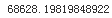
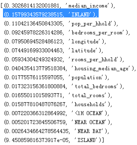
def display_scores(scores):
print("Scores:", scores)
print("Mean:", scores.mean())
print("Standard deviation:", scores.std())
display_scores(tree_rmse_scores)

Now the Decision Tree doesn’t look as good as it did earlier. In fact, it seems to perform worse(Mean RMSE=70644.94463282847) than the Linear Regression model(RMSE=68628.19819848922 see previous result, Mean RMSE=69052.46136345083, see belowing result)! Notice that cross-validation allows you to get not only an estimate of the performance of your model, but also a measure of how precise this estimate is (i.e., its standard deviation). The Decision Tree has a score of approximately 70645, generally ±2939. You would not have this information if you just used one validation set(housing_label). But cross-validation comes at the cost of training the model several times, so it is not always possible.
Let’s compute the same scores for the Linear Regression model just to be sure:
lin_scores = cross_val_score(lin_reg, housing_prepared, housing_label, scoring="neg_mean_squared_error", cv=10)
lin_rmse_scores = np.sqrt(-lin_scores)
display_scores(lin_rmse_scores)
That’s right: the Decision Tree model is overfitting so badly that it performs worse than the Linear Regression model.
Let’s try one last model now: the RandomForestRegressor. As we will see in Chapter 7, Random Forests work by training many Decision Trees on random subsets of the features, then averaging out their predictions. Building a model on top of many other models is called Ensemble Learning集成学习, and it is often a great way to push ML algorithms even further. We will skip most of the code since it is essentially the same as for the other models:
from sklearn.ensemble import RandomForestRegressor

forest_reg = RandomForestRegressor(n_estimators=100, random_state=42)
forest_reg.fit(housing_prepared, housing_label)

housing_predictions = forest_reg.predict(housing_prepared)
forest_mse = mean_squared_error(housing_label, housing_predictions)
forest_rmse = np.sqrt(forest_mse)
forest_rmse#one validation set(housing_label)
 #seems better
from sklearn.model_selection import cross_val_score
forest_scores = cross_val_score(forest_reg, housing_prepared, housing_label, \
scoring="neg_mean_squared_error", cv=10)
forest_rmse_scores = np.sqrt(-forest_scores)
display_scores(forest_rmse_scores)

Wow, this is much better: Random Forests look very promising. However, note that the score on the training set(18604.03726255338) is still much lower than on the validation sets(50182.027794261485), meaning that the model is still overfitting the training set. Possible solutions for overfitting are to simplify the model, constrain it (i.e., regularize it), or get a lot more training data. However, before you dive much deeper in Random Forests, you should try out many other models from various categories of Machine Learning algorithms (several Support Vector Machines with different kernels, possibly a neural network, etc.), without spending too much time tweaking调节 the hyperparameters. The goal is to shortlist a few (two to five) promising models.
Suport Vector Regression
from sklearn.svm import SVR
svm_reg = SVR(kernel='linear')
svm_reg.fit(housing_prepared, housing_label)
housing_predictions = svm_reg.predict(housing_prepared)
svm_mse = mean_squared_error(housing_label, housing_predictions)
svm_rmse = np.sqrt(svm_mse)
svm_rmse

################
TIP
You should save every model you experiment with, so you can come back easily to any model you want. Make sure you save
both the hyperparameters and the trained parameters, as well as the cross-validation scores and perhaps the actual predictions as well. This will allow you to easily compare scores across model types, and compare the types of errors they make. You can easily save Scikit-Learn models by using Python’s pickle module, or using sklearn.externals.joblib, which is more efficient at serializing large NumPy arrays:
from sklearn.externals import joblib
joblib.dump(my_model, "my_model.pkl")
# and later...
my_model_loaded = joblib.load("my_model.pkl")
VS:
scores = cross_val_score(lin_reg, housing_prepared, housing_label, scoring='neg_mean_squared_error', cv=10)
pd.Series(np.sqrt(-scores)).describe()

################
Grid Search
One way to do that would be to fiddle篡改 with the hyperparameters manually, until you find a great combination of hyperparameter values. This would be very tedious work, and you may not have time to explore many combinations.
Instead you should get Scikit-Learn’s GridSearchCV to search for you. All you need to do is tell it which hyperparameters you want it to experiment with, and what values to try out, and it will evaluate all the possible combinations of hyperparameter values, using cross-validation. For example, the following code searches for the best combination of hyperparameter values for the RandomForestRegressor:
#######################
Tip:
When you have no idea what value a hyperparameter should have, a simple approach is to try out consecutive powers of 10 (or a smaller number if you want a more fine-grained search, as shown in this example with the n_estimators hyperparameter).
#######################
from sklearn.model_selection import GridSearchCV
#All in all, the grid search will explore 12 + 6 = 18 combinations of RandomForestRegressor hyperparameter values,
param_grid = [
#This param_grid tells Scikit-Learn to first evaluate all 3 × 4 = 12
#combinations of n_estimators and max_features hyperparameter values specified in the first dict
{'n_estimators': [3,10,30], 'max_features':[2,4,6,8]},
#then try all 2 × 3 = 6 combinations of hyperparameter values in the second dict,
#but this time with the bootstrap hyperparameter set to False instead of
#True (which is the default value for this hyperparameter).
{'bootstrap': [False], 'n_estimators':[3,10], 'max_features':[2,3,4]}
]
forest_reg = RandomForestRegressor()
#it will train each model five times (since we are using five-fold cross validation).
#In other words, all in all, there will be 18 × 5 = 90 rounds of training!
grid_search = GridSearchCV(forest_reg, param_grid, cv=5, scoring='neg_mean_squared_error')
grid_search.fit(housing_prepared, housing_label)

grid_search.best_params_

Since 30 is the maximum value of n_estimators that was evaluated, you should probably evaluate higher values as well, since the score may continue to improve.
grid_search.best_estimator_

##############################
NOTE:
If GridSearchCV is initialized with refit=True (which is the default), then once it finds the best estimator using crossvalidation, it retrains it on the whole training set. This is usually a good idea since feeding it more data will likely improve its performance.
##############################
And of course the evaluation scores are also available:
cvres = grid_search.cv_results_
for mean_score, params in zip(cvres['mean_test_score'], cvres['params']):
print(np.sqrt(-mean_score), params)

In this example, we obtain the best solution by setting the max_features hyperparameter to 6, and the n_estimators hyperparameter to 30. The RMSE score for this combination is 50,010, which is slightly better than the score you got earlier using the default hyperparameter values without param_grid (which was 50182;
#################
from sklearn.model_selection import cross_val_score
forest_scores = cross_val_score(forest_reg, housing_prepared, housing_label, \
scoring="neg_mean_squared_error", cv=10)
forest_rmse_scores = np.sqrt(-forest_scores)
display_scores(forest_rmse_scores)
#################
Congratulations, you have successfully fine-tuned your best model!
############################
TIP
Don’t forget that you can treat some of the data preparation steps as hyperparameters. For example, the grid search will
automatically find out whether or not to add a feature you were not sure about (e.g., using the add_bedrooms_per_room
hyperparameter of your CombinedAttributesAdder transformer). It may similarly be used to automatically find the best way to handle outliers, missing features, feature selection, and more.
############################
Randomized Search
The grid search approach is fine when you are exploring relatively few combinations, like in the previous example, but when the hyperparameter search space is large, it is often preferable to use RandomizedSearchCV instead. This class can be used in much the same way as the GridSearchCV class, but instead of trying out all possible combinations,
it evaluates a given number of random combinations by selecting a random value for each hyperparameter at every iteration. This approach has two main benefits:
- If you let the randomized search run for, say, 1,000 iterations, this approach will explore 1,000 different values for each hyperparameter (instead of just a few values per hyperparameter with the grid search approach).
- You have more control over the computing budget you want to allocate to hyperparameter search, simply by setting the number of iterations.
Ensemble Methods
Another way to fine-tune your system is to try to combine the models that perform best. The group (or “ensemble”) will often perform better than the best individual model (just like Random Forests perform better than the individual Decision Trees
they rely on), especially if the individual models make very different types of errors.
Analyze the Best Models and Their Errors
You will often gain good insights on the problem by inspecting the best models. For example, the RandomForestRegressor can indicate the relative importance of each attribute for making accurate predictions:
feature_importances = grid_search.best_estimator_.feature_importances_
feature_importances

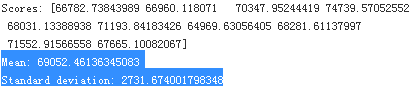
Let’s display these importance scores next to their corresponding attribute names:
extra_attribs = ["rooms_per_hhold", "pop_per_hhold", "bedrooms_per_room"]
cat_one_hot_attribs = list(encoder.classes_)
attributes = num_attribs + extra_attribs + cat_one_hot_attribs
sorted(zip(feature_importances, attributes), reverse=True)
With this information, you may want to try dropping some of the less useful features (e.g., apparently only
one ocean_proximity category is really useful, so you could try dropping the others).
You should also look at the specific errors that your system makes, then try to understand why it makes
them and what could fix the problem (adding extra features or, on the contrary, getting rid of uninformative
ones, cleaning up outliers, etc.).
Evaluate Your System on the Test Set
After tweaking your models for a while, you eventually have a system that performs sufficiently well. Now is the time to evaluate the final model on the test set. There is nothing special about this process; just get the predictors and the labels from your test set, run your full_pipeline to transform the data (call transform(), not fit_transform()!), and evaluate the final model on the test set:
final_model = grid_search.best_estimator_
X_test = strat_test_set.drop("median_house_value", axis=1)
y_test = strat_test_set["median_house_value"].copy()
X_test_prepared = full_pipeline.transform(X_test)
final_predictions = final_model.predict(X_test_prepared)
final_mse = mean_squared_error(y_test, final_predictions)
final_rmse = np.sqrt(final_mse)
final_rmse

The performance will usually be slightly worse than what you measured using cross-validation if you did a lot of hyperparameter tuning (because your system ends up fine-tuned to perform well on the validation data, and will likely not perform as well on unknown datasets). It is not the case in this example, but when this happens you must resist the temptation to tweak the hyperparameters to make the numbers look good on the test set; the improvements would be unlikely to generalize to new data.
We can compute a 95% confidence interval for the test RMSE:
the Root Mean Square Error (RMSE). It measures the standard deviation of the errors the system makes in its predictions. For example, an RMSE equal to 50,000 means that about 68% of the system’s predictions fall within $50,000 of the actual value, and about 95% of the predictions fall within $100,000 of the actual value. Equation 2-1 shows the mathematical formula to compute the RMSE.
When a feature has a bell-shaped normal distribution (also called a Gaussian distribution), which is very common,
the “68-95-99.7” rule applies: about 68% of the values fall within 1σ of the mean, 95% within 2σ, and 99.7% within 3σ.
from scipy import stats
confidence = 0.95
#residual=yi-y_hat_i
squared_errors = (final_predictions - y_test)**2
np.sqrt( stats.t.interval(confidence,
len(squared_errors)-1, #df=degrees of freedom=number of samples -1
loc = squared_errors.mean(), #the sample means
scale = stats.sem(squared_errors) #the standard error of the mean of the samples
)
)

##########################
stats.sem(squared_errors)


squared_errors_standard_deviation = np.sqrt( np.sum( ( np.array(squared_errors).reshape(length,1) - \
np.tile([squared_errors_mean],[1, length]).T
)**2
)/(length-1)
)
standard_error_of_mean=squared_errors_standard_deviation/np.sqrt(length)
standard_error_of_mean #for Square Errors
confidence = 0.95
(1-confidence)/2=


1.96 is actually an approximation
standard_error_of_mean=squared_errors_standard_deviation/np.sqrt(length)

##########################
Now comes the project prelaunch phase: you need to present your solution (highlighting what you have learned, what worked and what did not, what assumptions were made, and what your system’s limitations are), document everything, and create nice presentations with clear visualizations and easy-to-remember statements (e.g., “the median income is the number one predictor of housing prices”).
Launch, Monitor, and Maintain Your System
Perfect, you got approval to launch! You need to get your solution ready for production, in particular by plugging the production input data sources into your system and writing tests.
You also need to write monitoring code to check your system’s live performance at regular intervals and trigger alerts when it drops. This is important to catch not only sudden breakage, but also performance degradation. This is quite common because models tend to “rot” as data evolves over time, unless the models are regularly trained on fresh data.
Evaluating your system’s performance will require sampling the system’s predictions and evaluating them. This will generally require a human analysis. These analysts may be field experts, or workers on a crowdsourcing platform (such as Amazon Mechanical Turk or CrowdFlower). Either way, you need to plug the human evaluation pipeline into your system.
You should also make sure you evaluate the system’s input data quality. Sometimes performance will degrade slightly because of a poor quality signal (e.g., a malfunctioning sensor sending random values, or another team’s output becoming stale), but it may take a while before your system’s performance degrades enough to trigger an alert. If you monitor your system’s inputs, you may catch this earlier. Monitoring the inputs is particularly important for online learning systems.
Finally, you will generally want to train your models on a regular basis using fresh data. You should automate this process as much as possible. If you don’t, you are very likely to refresh your model only every six months (at best), and your system’s performance may fluctuate severely over time. If your system is an online learning system, you should make sure you save snapshots of its state at regular intervals so you can easily roll back to a previously working state.
02_End-to-End Machine Learning Project_03_stats.sem_ppf_CategoricalEncoder_RandomizedSearchCV_joblib
https://blog.csdn.net/Linli522362242/article/details/103646927