与MNIST类似,CIFAR-10同样是人工智能学习入门的数据集之一,它包含飞机、汽车、小鸟等10个类别的图片,一共60000张图片,其中训练集占50000张,测试集占10000张。
这里采用CNN网络对CIFAR-10数据集进行分类识别。
1 导入需要的模块
首先,导入需要用到的模块
import numpy as np

import tensorflow as tf
from tensorflow import keras
from keras import models, layers

import matplotlib.pyplot as plt
2 载入数据
利用keras集成的数据集载入CIFAR-10数据集
(train_images, train_labels), (test_images, test_labels) = keras.datasets.cifar10.load_data()
train_input = train_images.astype('float32')/255
test_input = test_images.astype('float32')/255
train_output = train_labels.astype('int16')
test_output = test_labels.astype('int16')
调用格式和mnist相同。生成train_images、train_labels、test_images、test_labels等四个变量,分别代表训练和测试图像和标记。其中图像数据的维度为Nx32x32x3,表示每张图片为32x32的彩色图片,每一个像素点由一个3维数据表示颜色。这里进行数据处理,把图像数据归一到0-1之间的浮点数。
3 构建模型
构建一个多层的CNN网络,定义构建函数
def build_model():
model = models.Sequential()
model.add(layers.Conv2D(16, (3,3), padding='same', activation='relu', data_format='channels_last', input_shape=(32,32,3)))
model.add(layers.Conv2D(16, (3,3), padding='same', activation='relu'))
model.add(layers.MaxPooling2D((2,2)))
model.add(layers.Conv2D(32, (3,3), padding='same', activation='relu'))
model.add(layers.Conv2D(32, (3,3), padding='same', activation='relu'))
model.add(layers.MaxPooling2D((2,2)))
model.add(layers.Flatten())
model.add(layers.Dense(128, activation='relu'))
model.add(layers.Dense(10, activation='softmax'))
model.compile(optimizer='adam',loss='sparse_categorical_crossentropy',metrics=['sparse_categorical_accuracy'])
return model
构建模型如下
network = build_model()
network.summary()
输出模型的结构,如下
Model: "sequential"
_________________________________________________________________
Layer (type)                 Output Shape              Param #
=================================================================
conv2d (Conv2D)              (None, 32, 32, 16)        448
_________________________________________________________________
conv2d_1 (Conv2D)            (None, 32, 32, 16)        2320
_________________________________________________________________
max_pooling2d (MaxPooling2D) (None, 16, 16, 16)        0
_________________________________________________________________
conv2d_2 (Conv2D)            (None, 16, 16, 32)        4640
_________________________________________________________________
conv2d_3 (Conv2D)            (None, 16, 16, 32)        9248
_________________________________________________________________
max_pooling2d_1 (MaxPooling2 (None, 8, 8, 32)          0
_________________________________________________________________
flatten (Flatten)            (None, 2048)              0
_________________________________________________________________
dense (Dense)                (None, 128)               262272
_________________________________________________________________
dense_1 (Dense)              (None, 10)                1290
=================================================================
Total params: 280,218
Trainable params: 280,218
Non-trainable params: 0
4 训练模型
调用训练模型函数
history = network.fit(train_input, train_output, epochs=20, batch_size=64, validation_split=0.2)
显示结果
Epoch 1/20
625/625 [==============================] - 6s 5ms/step - loss: 1.5318 - sparse_categorical_accuracy: 0.4451 - val_loss: 1.2786 - val_sparse_categorical_accuracy: 0.5455
Epoch 2/20
625/625 [==============================] - 2s 4ms/step - loss: 1.1113 - sparse_categorical_accuracy: 0.6072 - val_loss: 1.0753 - val_sparse_categorical_accuracy: 0.6193
Epoch 3/20
625/625 [==============================] - 2s 4ms/step - loss: 0.9271 - sparse_categorical_accuracy: 0.6734 - val_loss: 0.9335 - val_sparse_categorical_accuracy: 0.6716
Epoch 4/20
625/625 [==============================] - 2s 4ms/step - loss: 0.8096 - sparse_categorical_accuracy: 0.7171 - val_loss: 0.8828 - val_sparse_categorical_accuracy: 0.6968
Epoch 5/20
625/625 [==============================] - 2s 4ms/step - loss: 0.7269 - sparse_categorical_accuracy: 0.7457 - val_loss: 0.8725 - val_sparse_categorical_accuracy: 0.7000

...
Epoch 19/20
625/625 [==============================] - 2s 4ms/step - loss: 0.0986 - sparse_categorical_accuracy: 0.9653 - val_loss: 1.8485 - val_sparse_categorical_accuracy: 0.7065
Epoch 20/20
625/625 [==============================] - 2s 4ms/step - loss: 0.0917 - sparse_categorical_accuracy: 0.9673 - val_loss: 1.9127 - val_sparse_categorical_accuracy: 0.7050
训练过程的变量包含在返回变量history中,绘制训练过程如下
loss = history.history['loss']
val_loss = history.history['val_loss']
acc = history.history['sparse_categorical_accuracy']
val_acc = history.history['val_sparse_categorical_accuracy']
plt.figure(figsize=(10,3))
plt.subplot(1,2,1)
plt.plot(loss, color='blue', label='train')
plt.plot(val_loss, color='red', label='test')
plt.ylabel('loss')
plt.legend()
plt.subplot(1,2,2)
plt.plot(acc, color='blue', label='train')
plt.plot(val_acc, color='red', label='test')
plt.ylabel('accuracy')
plt.legend()
显示结果如下
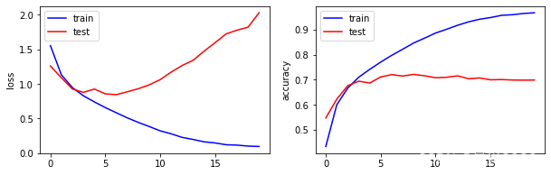
分别绘制了训练阶段和测试阶段的分类识别精度和损失函数,蓝线表示训练阶段的损失函数和准确度,红线表示测试阶段的损失函数和准确度。结果显示通过训练,神经网络模型在训练集上的表现性能越来越好,但是在测试集上的识别准确度并没有提升,相反损失函数反而变大。说面模型训练出现过拟合的情况,泛化能力较差。
5 评估模型
评估训练后模型的性能,如下
network.evaluate(test_input, test_output, verbose=2)
显示结果
313/313 - 1s - loss: 2.0248 - sparse_categorical_accuracy: 0.6923
[2.02479887008667, 0.692300021648407]
在测试集上的准确度为0.6923。
在这里绘制测试集前100张图片的识别结果
predict_output = network.predict(test_input)
m = 10
n = 10
num = m*n
labels = ['airplane', 'automobile', 'bird', 'cat', 'deer', 'dog', 'frog', 'horse', 'ship', 'truck']
plt.figure(figsize=(15,15))
for i in range(num):
plt.subplot(m,n,i+1)
type_index = np.argmax(predict_output[i]);
label = labels[type_index]
clr = 'black' if type_index == test_labels[i] else 'red'
plt.imshow(test_images[i])
plt.xticks([])
plt.yticks([])
plt.xlabel(label, color=clr)
plt.show()
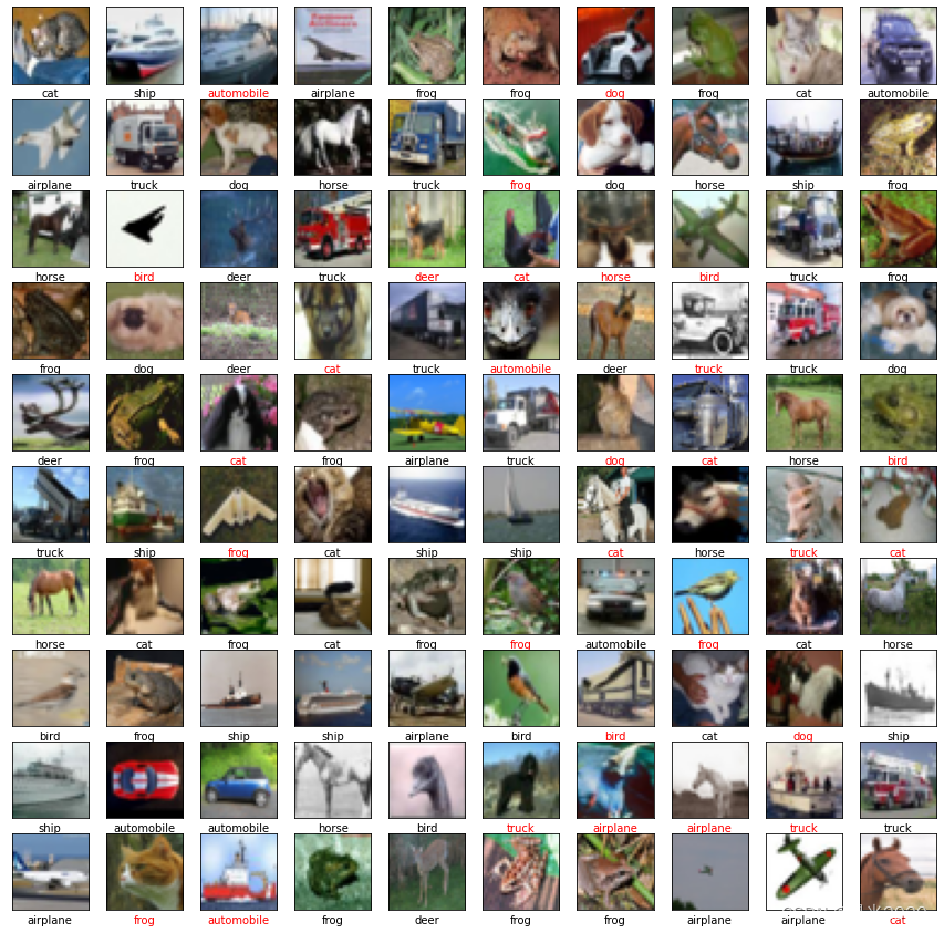
黑色字体表示正确的识别,红色字体表示错误的识别,结果显示,在测试集前100张图片的识别中,大概还有30%左右的误识别率。也证明了前面的评估结果。说明了这个模型的泛化能力不足。还需要优化模型参数和结构。
参考链接:https://blog.csdn.net/weixin_45954454/article/details/114519299
本文内容由网友自发贡献,版权归原作者所有,本站不承担相应法律责任。如您发现有涉嫌抄袭侵权的内容,请联系:hwhale#tublm.com(使用前将#替换为@)