DICOM是医学图像中标准文件,这些文件包含了诸多的元数据信息(比如像素尺寸,每个维度的一像素代表真实世界里的长度)。此处以kaggle Data Science Bowl 数据集为例。
data-science-bowl-2017。数据列表如下:
后缀为 .dcm。
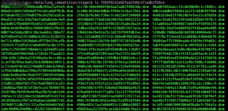
每个病人的一次扫描CT(scan)可能有几十到一百多个dcm数据文件(slices)。可以使用 python的dicom包读取,读取示例代码如下:
dicom.read_file('/data/lung_competition/stage1/7050f8141e92fa42fd9c471a8b2f50ce/498d16aa2222d76cae1da144ddc59a13.dcm')
其pixl_array包含了真实数据。
slices = [dicom.read_file(os.path.join(folder_name,filename)) for filename in os.listdir(folder_name)]
slices = np.stack([s.pixel_array for s in slices])
mhd格式是另外一种数据格式,来源于(LUNA2016)[https://luna16.grand-challenge.org/data/]。每个病人一个mhd文件和一个同名的raw文件。如下:
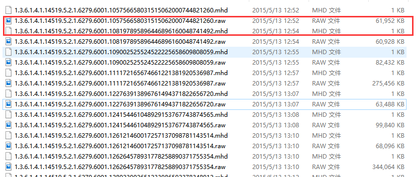
一个mhd通常有几百兆,对应的raw文件只有1kb。mhd文件需要借助python的SimpleITK包来处理。SimpleITK 示例代码如下:
import SimpleITK as sitk
itk_img = sitk.ReadImage(img_file)
img_array = sitk.GetArrayFromImage(itk_img) # indexes are z,y,x (notice the ordering)
num_z, height, width = img_array.shape        #heightXwidth constitute the transverse plane
origin = np.array(itk_img.GetOrigin())      # x,y,z  Origin in world coordinates (mm)
spacing = np.array(itk_img.GetSpacing())    # spacing of voxels in world coor. (mm)
需要注意的是,SimpleITK的img_array的数组不是直接的像素值,而是相对于CT扫描中原点位置的差值,需要做进一步转换。转换步骤参考 SimpleITK图像转换
一个开源免费的查看软件 mango
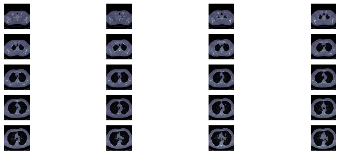
首先,需要明白的是医学扫描图像(scan)其实是三维图像,使用代码读取之后开源查看不同的切面的切片(slices),可以从不同轴切割
如下图展示了一个病人CT扫描图中,其中部分切片slices
其次,CT扫描图是包含了所有组织的,如果直接去看,看不到任何有用信息。需要做一些预处理,预处理中一个重要的概念是放射剂量,衡量单位为HU(Hounsfield Unit),下表是不同放射剂量对应的组织器官
| substance |
HU |
| 空气 |
-1000 |
| 肺 |
-500 |
| 脂肪 |
-100到-50 |
| 水 |
0 |
| CSF |
15 |
| 肾 |
30 |
| 血液 |
+30到+45 |
| 肌肉 |
+10到+40 |
| 灰质 |
+37到+45 |
| 白质 |
+20到+30 |
| Liver |
+40到+60 |
| 软组织,constrast |
+100到+300 |
| 骨头 |
+700(软质骨)到+3000(皮质骨) |
Hounsfield Unit = pixel_value * rescale_slope + rescale_intercept
一般情况rescale slope = 1, intercept = -1024。
上表中肺部组织的HU数值为-500,但通常是大于这个值,比如-320、-400。挑选出这些区域,然后做其他变换抽取出肺部像素点。
2.2 先载入必要的包
# -*- coding:utf-8 -*-
'''
this script is used for basic process of lung 2017 in Data Science Bowl
'''
import glob
import os
import pandas as pd
import SimpleITK as sitk
import numpy as np # linear algebra
import pandas as pd # data processing, CSV file I/O (e.g. pd.read_csv)
import skimage, os
from skimage.morphology import ball, disk, dilation, binary_erosion, remove_small_objects, erosion, closing, reconstruction, binary_closing
from skimage.measure import label,regionprops, perimeter
from skimage.morphology import binary_dilation, binary_opening
from skimage.filters import roberts, sobel
from skimage import measure, feature
from skimage.segmentation import clear_border
from skimage import data
from scipy import ndimage as ndi
import matplotlib
#matplotlib.use('Agg')
import matplotlib.pyplot as plt
from mpl_toolkits.mplot3d.art3d import Poly3DCollection
import dicom
import scipy.misc
import numpy as np
如下代码是载入一个扫描面,包含了多个切片(slices),我们仅简化的将其存储为python列表。数据集中每个目录都是一个扫描面集(一个病人)。有个元数据域丢失,即Z轴方向上的像素尺寸,也即切片的厚度 。所幸,我们可以用其他值推测出来,并加入到元数据中。
# Load the scans in given folder path
def load_scan(path):
    slices = [dicom.read_file(path + '/' + s) for s in os.listdir(path)]
    slices.sort(key = lambda x: int(x.ImagePositionPatient[2]))
    try:
        slice_thickness = np.abs(slices[0].ImagePositionPatient[2] - slices[1].ImagePositionPatient[2])
    except:
        slice_thickness = np.abs(slices[0].SliceLocation - slices[1].SliceLocation)
    for s in slices:
        s.SliceThickness = slice_thickness
    return slices
首先去除灰度值为 -2000的pixl_array,CT扫描边界之外的灰度值固定为-2000(dicom和mhd都是这个值)。第一步是设定这些值为0,当前对应为空气(值为0)
回到HU单元,乘以rescale比率并加上intercept(存储在扫描面的元数据中)。
def get_pixels_hu(slices):
    image = np.stack([s.pixel_array for s in slices])
    # Convert to int16 (from sometimes int16),
    # should be possible as values should always be low enough (<32k)
    image = image.astype(np.int16)
    # Set outside-of-scan pixels to 0
    # The intercept is usually -1024, so air is approximately 0
    image[image == -2000] = 0
    # Convert to Hounsfield units (HU)
    for slice_number in range(len(slices)):
        intercept = slices[slice_number].RescaleIntercept
        slope = slices[slice_number].RescaleSlope
        if slope != 1:
            image[slice_number] = slope * image[slice_number].astype(np.float64)
            image[slice_number] = image[slice_number].astype(np.int16)
        image[slice_number] += np.int16(intercept)
    return np.array(image, dtype=np.int16)
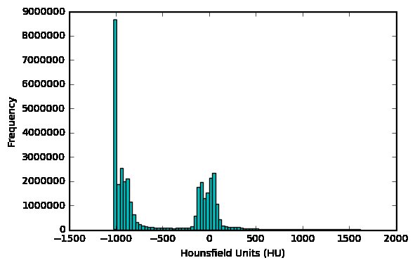
可以查看病人的扫描HU值分布情况
first_patient = load_scan(INPUT_FOLDER + patients[0])
first_patient_pixels = get_pixels_hu(first_patient)
plt.hist(first_patient_pixels.flatten(), bins=80, color='c')
plt.xlabel("Hounsfield Units (HU)")
plt.ylabel("Frequency")
plt.show()
不同扫描面的像素尺寸、粗细粒度是不同的。这不利于我们进行CNN任务,我们可以使用同构采样。
一个扫描面的像素区间可能是[2.5,0.5,0.5],即切片之间的距离为2.5mm。可能另外一个扫描面的范围是[1.5,0.725,0.725]。这可能不利于自动分析。
常见的处理方法是从全数据集中以固定的同构分辨率重新采样,将所有的东西采样为1mmx1mmx1mm像素。
def resample(image, scan, new_spacing=[1,1,1]):
    # Determine current pixel spacing
    spacing = map(float, ([scan[0].SliceThickness] + scan[0].PixelSpacing))
    spacing = np.array(list(spacing))
    resize_factor = spacing / new_spacing
    new_real_shape = image.shape * resize_factor
    new_shape = np.round(new_real_shape)
    real_resize_factor = new_shape / image.shape
    new_spacing = spacing / real_resize_factor
    image = scipy.ndimage.interpolation.zoom(image, real_resize_factor, mode='nearest')
    return image, new_spacing
现在重新取样病人的像素,将其映射到一个同构分辨率 1mm x1mm x1mm。
pix_resampled, spacing = resample(first_patient_pixels, first_patient, [1,1,1])
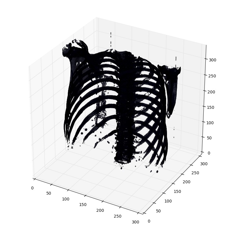
使用matplotlib输出肺部扫描的3D图像方法。可能需要一两分钟。
def plot_3d(image, threshold=-300):
    # Position the scan upright,
    # so the head of the patient would be at the top facing the camera
    p = image.transpose(2,1,0)
    verts, faces = measure.marching_cubes(p, threshold)
    fig = plt.figure(figsize=(10, 10))
    ax = fig.add_subplot(111, projection='3d')
    # Fancy indexing: `verts[faces]` to generate a collection of triangles
    mesh = Poly3DCollection(verts[faces], alpha=0.1)
    face_color = [0.5, 0.5, 1]
    mesh.set_facecolor(face_color)
    ax.add_collection3d(mesh)
    ax.set_xlim(0, p.shape[0])
    ax.set_ylim(0, p.shape[1])
    ax.set_zlim(0, p.shape[2])
    plt.show()
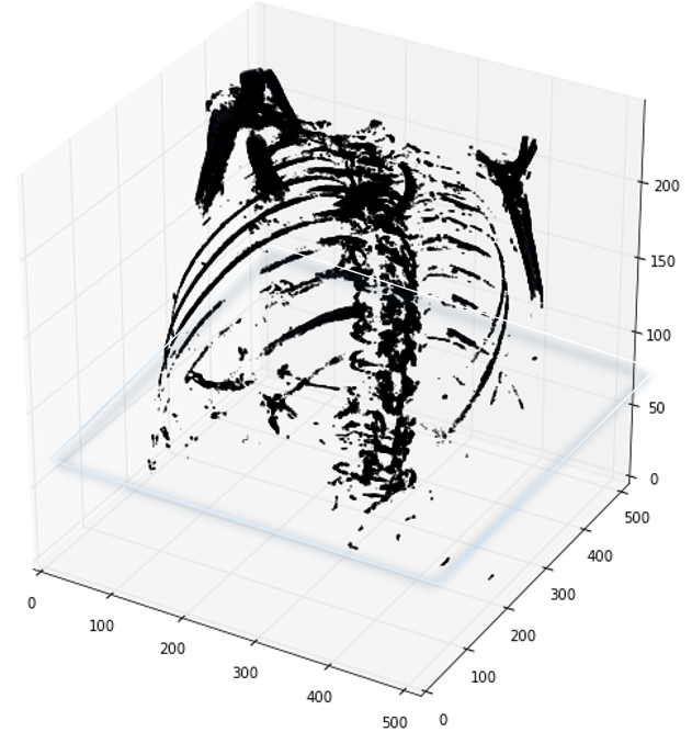
打印函数有个阈值参数,来打印特定的结构,比如tissue或者骨头。400是一个仅仅打印骨头的阈值(HU对照表)
plot_3d(pix_resampled, 400)
def plot_ct_scan(scan):
    '''
            plot a few more images of the slices
    :param scan:
    :return:
    '''
    f, plots = plt.subplots(int(scan.shape[0] / 20) + 1, 4, figsize=(50, 50))
    for i in range(0, scan.shape[0], 5):
        plots[int(i / 20), int((i % 20) / 5)].axis('off')
        plots[int(i / 20), int((i % 20) / 5)].imshow(scan[i], cmap=plt.cm.bone)
此方法的效果示例如下:

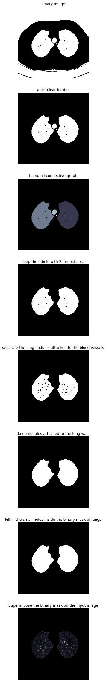
下面的代码使用了pythonde 的图像形态学操作。具体可以参考python高级形态学操作
def get_segmented_lungs(im, plot=False):
    '''
    This funtion segments the lungs from the given 2D slice.
    '''
    if plot == True:
        f, plots = plt.subplots(8, 1, figsize=(5, 40))
    '''
    Step 1: Convert into a binary image.
    '''
    binary = im < 604
    if plot == True:
        plots[0].axis('off')
        plots[0].set_title('binary image')
        plots[0].imshow(binary, cmap=plt.cm.bone)
    '''
    Step 2: Remove the blobs connected to the border of the image.
    '''
    cleared = clear_border(binary)
    if plot == True:
        plots[1].axis('off')
        plots[1].set_title('after clear border')
        plots[1].imshow(cleared, cmap=plt.cm.bone)
    '''
    Step 3: Label the image.
    '''
    label_image = label(cleared)
    if plot == True:
        plots[2].axis('off')
        plots[2].set_title('found all connective graph')
        plots[2].imshow(label_image, cmap=plt.cm.bone)
    '''
    Step 4: Keep the labels with 2 largest areas.
    '''
    areas = [r.area for r in regionprops(label_image)]
    areas.sort()
    if len(areas) > 2:
        for region in regionprops(label_image):
            if region.area < areas[-2]:
                for coordinates in region.coords:
                       label_image[coordinates[0], coordinates[1]] = 0
    binary = label_image > 0
    if plot == True:
        plots[3].axis('off')
        plots[3].set_title(' Keep the labels with 2 largest areas')
        plots[3].imshow(binary, cmap=plt.cm.bone)
    '''
    Step 5: Erosion operation with a disk of radius 2. This operation is
    seperate the lung nodules attached to the blood vessels.
    '''
    selem = disk(2)
    binary = binary_erosion(binary, selem)
    if plot == True:
        plots[4].axis('off')
        plots[4].set_title('seperate the lung nodules attached to the blood vessels')
        plots[4].imshow(binary, cmap=plt.cm.bone)
    '''
    Step 6: Closure operation with a disk of radius 10. This operation is
    to keep nodules attached to the lung wall.
    '''
    selem = disk(10)
    binary = binary_closing(binary, selem)
    if plot == True:
        plots[5].axis('off')
        plots[5].set_title('keep nodules attached to the lung wall')
        plots[5].imshow(binary, cmap=plt.cm.bone)
    '''
    Step 7: Fill in the small holes inside the binary mask of lungs.
    '''
    edges = roberts(binary)
    binary = ndi.binary_fill_holes(edges)
    if plot == True:
        plots[6].axis('off')
        plots[6].set_title('Fill in the small holes inside the binary mask of lungs')
        plots[6].imshow(binary, cmap=plt.cm.bone)
    '''
    Step 8: Superimpose the binary mask on the input image.
    '''
    get_high_vals = binary == 0
    im[get_high_vals] = 0
    if plot == True:
        plots[7].axis('off')
        plots[7].set_title('Superimpose the binary mask on the input image')
        plots[7].imshow(im, cmap=plt.cm.bone)
    return im
此方法每个步骤对图像做不同的处理,依次为二值化、清除边界、连通区域标记、腐蚀操作、闭合运算、孔洞填充、效果如下:
为了减少有问题的空间,我们可以分割肺部图像(有时候是附近的组织)。这包含一些步骤,包括区域增长和形态运算,此时,我们只分析相连组件。
步骤如下:
-
阈值图像(-320HU是个极佳的阈值,但是此方法中不是必要)
-
处理相连的组件,以决定当前患者的空气的标签,以1填充这些二值图像
-
可选:当前扫描的每个轴上的切片,选定最大固态连接的组织(当前患者的肉体和空气),并且其他的为0。以掩码的方式填充肺部结构。
-
只保留最大的气袋(人类躯体内到处都有气袋)
def largest_label_volume(im, bg=-1):
    vals, counts = np.unique(im, return_counts=True)
    counts = counts[vals != bg]
    vals = vals[vals != bg]
    if len(counts) > 0:
        return vals[np.argmax(counts)]
    else:
        return None
def segment_lung_mask(image, fill_lung_structures=True):
    # not actually binary, but 1 and 2.
    # 0 is treated as background, which we do not want
    binary_image = np.array(image > -320, dtype=np.int8)+1
    labels = measure.label(binary_image)
    # Pick the pixel in the very corner to determine which label is air.
    #   Improvement: Pick multiple background labels from around the patient
    #   More resistant to "trays" on which the patient lays cutting the air
    #   around the person in half
    background_label = labels[0,0,0]
    #Fill the air around the person
    binary_image[background_label == labels] = 2
    # Method of filling the lung structures (that is superior to something like
    # morphological closing)
    if fill_lung_structures:
        # For every slice we determine the largest solid structure
        for i, axial_slice in enumerate(binary_image):
            axial_slice = axial_slice - 1
            labeling = measure.label(axial_slice)
            l_max = largest_label_volume(labeling, bg=0)
            if l_max is not None: #This slice contains some lung
                binary_image[i][labeling != l_max] = 1
    binary_image -= 1 #Make the image actual binary
    binary_image = 1-binary_image # Invert it, lungs are now 1
    # Remove other air pockets insided body
    labels = measure.label(binary_image, background=0)
    l_max = largest_label_volume(labels, bg=0)
    if l_max is not None: # There are air pockets
        binary_image[labels != l_max] = 0
    return binary_image
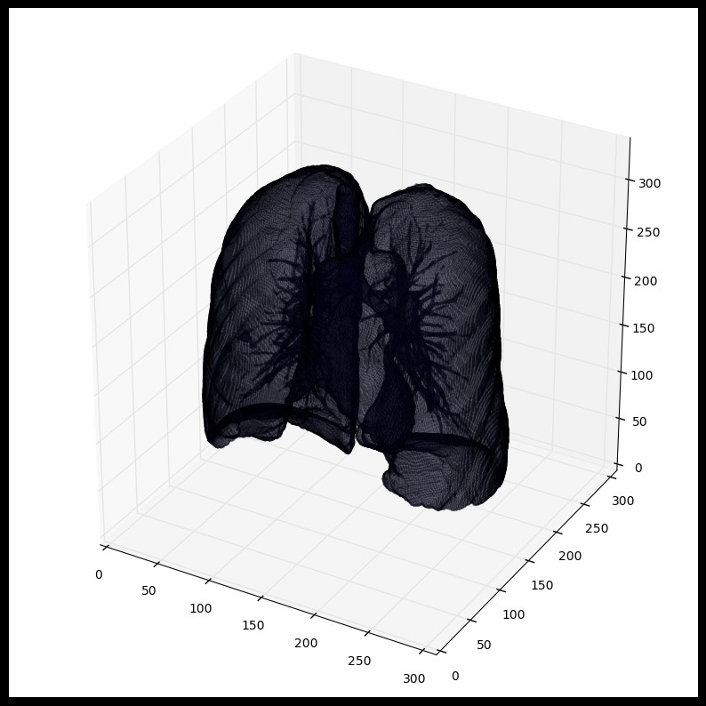
查看切割效果
segmented_lungs = segment_lung_mask(pix_resampled, False)
segmented_lungs_fill = segment_lung_mask(pix_resampled, True)
plot_3d(segmented_lungs, 0)
我们可以将肺内的结构也包含进来(结节是固体),不仅仅只是肺部内的空气
-
plot_3d(segmented_lungs_fill, 0)
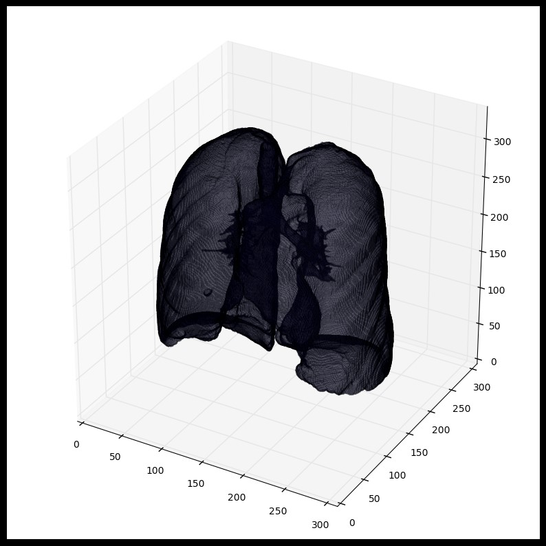
使用mask时,要注意首先进行形态扩充(python的skimage的skimage.morphology)操作(即使用圆形kernel,结节是球体),参考 python形态操作。这会在所有方向(维度)上扩充mask。仅仅肺部的空气+结构将不会包含所有结节,事实上有可能遗漏黏在肺部一侧的结节(这会经常出现,所以建议最好是扩充mask)。
归一化处理
当前的值范围是[-1024,2000]。而任意大于400的值并不是处理肺结节需要考虑,因为它们都是不同反射密度下的骨头。LUNA16竞赛中常用来做归一化处理的阈值集是-1000和400.以下代码
归一化
MIN_BOUND = -1000.0
MAX_BOUND = 400.0
def normalize(image):
    image = (image - MIN_BOUND) / (MAX_BOUND - MIN_BOUND)
    image[image>1] = 1.
    image[image<0] = 0.
    return image
0值中心化
简单来说就是所有像素值减去均值。LUNA16竞赛中的均值大约是0.25.
不要对每一张图像做零值中心化(此处像是在kernel中完成的)CT扫描器返回的是校准后的精确HU计量。不会出现普通图像中会出现某些图像低对比度和明亮度的情况
PIXEL_MEAN = 0.25
def zero_center(image):
    image = image - PIXEL_MEAN
    return image
归一化和零值中心化的操作主要是为了后续训练网络,零值中心化是网络收敛的关键。
mhd的数据只是格式与dicom不一样,其实质包含的都是病人扫描。处理MHD需要借助SimpleIKT这个包,处理思路详情可以参考Data Science Bowl2017的toturail Data Science Bowl 2017。需要注意的是MHD格式的数据没有HU值,它的值域范围与dicom很不同。
我们以LUNA2016年的数据处理流程为例。参考代码为 LUNA2016数据切割
import SimpleITK as sitk
import numpy as np
import csv
from glob import glob
import pandas as pd
file_list=glob(luna_subset_path+"*.mhd")
#####################
#
# Helper function to get rows in data frame associated
# with each file
def get_filename(case):
    global file_list
    for f in file_list:
        if case in f:
            return(f)
#
# The locations of the nodes
df_node = pd.read_csv(luna_path+"annotations.csv")
df_node["file"] = df_node["seriesuid"].apply(get_filename)
df_node = df_node.dropna()
#####
#
# Looping over the image files
#
fcount = 0
for img_file in file_list:
    print "Getting mask for image file %s" % img_file.replace(luna_subset_path,"")
    mini_df = df_node[df_node["file"]==img_file] #get all nodules associate with file
    if len(mini_df)>0:       # some files may not have a nodule--skipping those
        biggest_node = np.argsort(mini_df["diameter_mm"].values)[-1]   # just using the biggest node
        node_x = mini_df["coordX"].values[biggest_node]
        node_y = mini_df["coordY"].values[biggest_node]
        node_z = mini_df["coordZ"].values[biggest_node]
        diam = mini_df["diameter_mm"].values[biggest_node]
一直在寻找MHD格式数据的处理方法,对于dicom格式的CT有很多论文根据其HU值域可以轻易地分割肺、骨头、血液等,但是对于MHD没有这样的参考。从LUNA16论坛得到的解释是,LUNA16的MHD数据已经转换为HU值了,不需要再使用slope和intercept来做rescale变换了。此论坛主题下,有人提出MHD格式没有提供pixel spacing(mm) 和 slice thickness(mm) ,而标准文件annotation.csv文件中结节的半径和坐标都是mm单位,最后确认的是MHD格式文件中只保留了体素尺寸以及坐标原点位置,没有保存slice thickness。即,dicom才是原始数据格式。
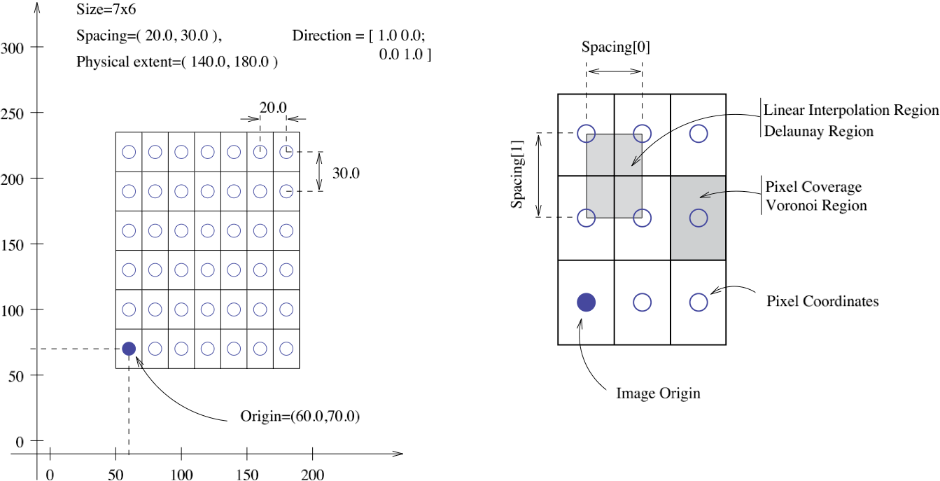
MHD值的坐标体系是体素,以mm为单位(dicom的值是GV灰度值)。结节的位置是CT scanner坐标轴里面相对原点的mm值,需要将其转换到真实坐标轴位置,可以使用SimpleITK包中的 GetOrigin() ` GetSpacing()`。图像数据是以512x512数组的形式给出的。
坐标变换如下:
相应的代码处理如下:
itk_img = sitk.ReadImage(img_file)
img_array = sitk.GetArrayFromImage(itk_img) # indexes are z,y,x (notice the ordering)
center = np.array([node_x,node_y,node_z])   # nodule center
origin = np.array(itk_img.GetOrigin())      # x,y,z  Origin in world coordinates (mm)
spacing = np.array(itk_img.GetSpacing())    # spacing of voxels in world coor. (mm)
v_center =np.rint((center-origin)/spacing)  # nodule center in voxel space (still x,y,z ordering)
在LUNA16的标注CSV文件中标注了结节中心的X,Y,Z轴坐标,但是实际取值的时候取的是Z轴最后三层的数组(img_array)。
下述代码只提取了包含结节的最后三个slice的数据,代码参考自 LUNA_mask_extraction.py
i = 0
for i_z in range(int(v_center[2])-1,int(v_center[2])+2):
    mask = make_mask(center,diam,i_z*spacing[2]+origin[2],width,height,spacing,origin)
    masks[i] = mask
    imgs[i] = matrix2int16(img_array[i_z])
    i+=1
np.save(output_path+"images_%d.npy" % (fcount) ,imgs)
np.save(output_path+"masks_%d.npy" % (fcount) ,masks)
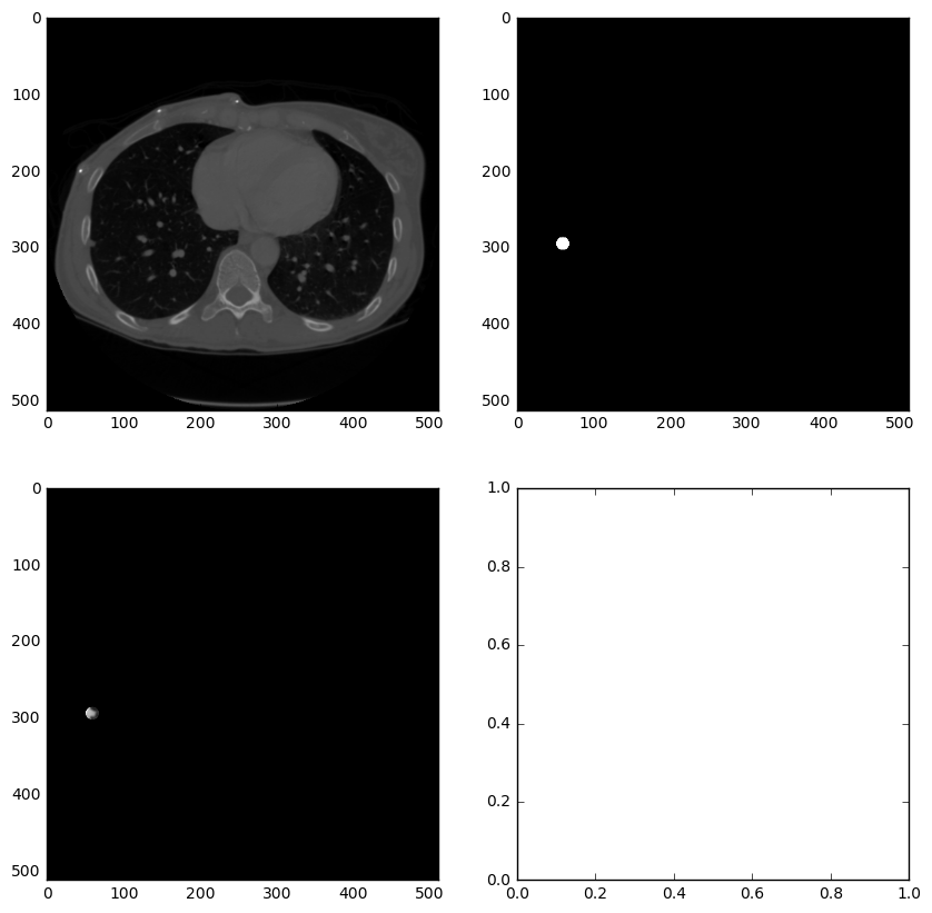
以下代码用于查看原始CT和结节mask。其实就是用matplotlib打印上一步存储的npy文件。
import matplotlib.pyplot as plt
imgs = np.load(output_path+'images_0.npy')
masks = np.load(output_path+'masks_0.npy')
for i in range(len(imgs)):
    print "image %d" % i
    fig,ax = plt.subplots(2,2,figsize=[8,8])
    ax[0,0].imshow(imgs[i],cmap='gray')
    ax[0,1].imshow(masks[i],cmap='gray')
    ax[1,0].imshow(imgs[i]*masks[i],cmap='gray')
    plt.show()
    raw_input("hit enter to cont : ")
接下来的处理和DICOM格式数据差不多,腐蚀膨胀、连通区域标记等。
参考信息:
灰度值是pixel value经过重重LUT转换得到的用来进行显示的值,而这个转换过程是不可逆的,也就是说,灰度值无法转换为ct值。只能根据窗宽窗位得到一个大概的范围。 pixel value经过modality lut得到Hu,但是怀疑pixelvalue的读取出了问题。dicom文件中存在(0028,0106)(0028,0107)两个tag,分别是最大最小pixel value,可以用来检验你读取的pixel value 矩阵是否正确。
LUT全称look up table,实际上就是一张像素灰度值的映射表,它将实际采样到的像素灰度值经过一定的变换如阈值、反转、二值化、对比度调整、线性变换等,变成了另外一 个与之对应的灰度值,这样可以起到突出图像的有用信息,增强图像的光对比度的作用。
参考:http://shartoo.github.io/medical_image_process/