GaussianNB就是先验为高斯分布(正态分布)的朴素贝叶斯,假设每个标签的数据都服从简单的正态分布。
P
(
X
j
=
x
j
∣
Y
=
C
k
)
=
1
2
π
σ
k
2
e
x
p
(
−
(
x
j
−
μ
k
)
2
2
σ
k
2
)
P(X_j=x_j|Y=C_k)=\frac{1}{\sqrt{2\pi\sigma^2_k}}exp\left(-\frac{(x_j-\mu_k)^2}{2\sigma^2_k}\right)
P(Xj=xj∣Y=Ck)=2πσk21exp(−2σk2(xj−μk)2) 其中
C
k
C_k
Ck为Y的第k类类别,
μ
k
\mu_k
μk和
σ
k
2
\sigma^2_k
σk2为需要从训练集估计的值
理解起来可能有点抽象,那我们从朴素贝叶斯的原理说起:
P
(
类
别
∣
特
征
)
=
P
(
特
征
∣
类
别
)
P
(
类
别
)
P
(
特
征
)
P(类别|特征)=\frac{P(特征|类别)P(类别)}{P(特征)}
P(类别∣特征)=P(特征)P(特征∣类别)P(类别)
进一步展开的话
P
(
′
I
r
i
s
−
s
e
t
o
s
a
′
∣
[
4.2
,
4.5
,
1.2
,
0.5
]
)
=
P
(
[
4.2
,
4.5
,
1.2
,
0.5
]
∣
′
I
r
i
s
−
s
e
t
o
s
a
′
)
P
(
′
I
r
i
s
−
s
e
t
o
s
a
′
)
P
[
4.2
,
4.5
,
1.2
,
0.5
]
P('Iris-setosa'|[4.2 , 4.5 , 1.2 , 0.5]) = \frac{P([4.2 , 4.5 , 1.2 , 0.5]|'Iris-setosa')P('Iris-setosa')}{P[4.2 , 4.5 , 1.2 , 0.5]}
P(′Iris−setosa′∣[4.2,4.5,1.2,0.5])=P[4.2,4.5,1.2,0.5]P([4.2,4.5,1.2,0.5]∣′Iris−setosa′)P(′Iris−setosa′)
P
(
′
I
r
i
s
−
v
e
r
s
i
c
o
l
o
r
′
∣
[
4.2
,
4.5
,
1.2
,
0.5
]
)
=
P
(
[
4.2
,
4.5
,
1.2
,
0.5
]
∣
′
I
r
i
s
−
v
e
r
s
i
c
o
l
o
r
′
)
P
(
′
I
r
i
s
−
v
e
r
s
i
c
o
l
o
r
′
)
P
[
4.2
,
4.5
,
1.2
,
0.5
]
P('Iris-versicolor'|[4.2 , 4.5 , 1.2 , 0.5]) = \frac{P([4.2 , 4.5 , 1.2 , 0.5]|'Iris-versicolor')P('Iris-versicolor')}{P[4.2 , 4.5 , 1.2 , 0.5]}
P(′Iris−versicolor′∣[4.2,4.5,1.2,0.5])=P[4.2,4.5,1.2,0.5]P([4.2,4.5,1.2,0.5]∣′Iris−versicolor′)P(′Iris−versicolor′)
P
(
′
I
r
i
s
−
v
i
r
g
i
n
i
c
a
′
∣
[
4.2
,
4.5
,
1.2
,
0.5
]
)
=
P
(
[
4.2
,
4.5
,
1.2
,
0.5
]
∣
′
I
r
i
s
−
v
i
r
g
i
n
i
c
a
′
)
P
(
′
′
I
r
i
s
−
v
i
r
g
i
n
i
c
a
′
)
P
[
4.2
,
4.5
,
1.2
,
0.5
]
P('Iris-virginica'|[4.2 , 4.5 , 1.2 , 0.5]) = \frac{P([4.2 , 4.5 , 1.2 , 0.5]|'Iris-virginica')P(''Iris-virginica')}{P[4.2 , 4.5 , 1.2 , 0.5]}
P(′Iris−virginica′∣[4.2,4.5,1.2,0.5])=P[4.2,4.5,1.2,0.5]P([4.2,4.5,1.2,0.5]∣′Iris−virginica′)P(′′Iris−virginica′)
接下来就剩P([4.2 , 4.5 , 1.2 , 0.5]|‘Iris-virginica’)的求解了。 在求解之前,因为朴素贝叶斯假设各特征之间都是独立的,所以
P
(
[
4.2
,
4.5
,
1.2
,
0.5
]
∣
′
I
r
i
s
−
v
i
r
g
i
n
i
c
a
′
)
=
P
(
f
e
a
t
u
r
e
0
=
4.2
∣
′
I
r
i
s
−
s
e
t
o
s
a
′
)
P
(
f
e
a
t
u
r
e
1
=
4.5
∣
′
I
r
i
s
−
s
e
t
o
s
a
′
)
P
(
f
e
a
t
u
r
e
2
=
1.2
∣
′
I
r
i
s
−
s
e
t
o
s
a
′
)
P
(
f
e
a
t
u
r
e
3
=
0.5
∣
′
I
r
i
s
−
s
e
t
o
s
a
′
)
P([4.2 , 4.5 , 1.2 , 0.5]|'Iris-virginica')=P(feature0=4.2|'Iris-setosa')P(feature1=4.5|'Iris-setosa')P(feature2=1.2|'Iris-setosa')P(feature3=0.5|'Iris-setosa')
P([4.2,4.5,1.2,0.5]∣′Iris−virginica′)=P(feature0=4.2∣′Iris−setosa′)P(feature1=4.5∣′Iris−setosa′)P(feature2=1.2∣′Iris−setosa′)P(feature3=0.5∣′Iris−setosa′) 我们以等号右边的P(feature0=4.2|‘Iris-setosa’)为例,讲解求解过程,这个会了其他的就都会啦 GaussianNB假设每个特征是符合高斯分布的,所以
P
(
f
e
a
t
u
r
e
0
=
4.2
∣
′
I
r
i
s
−
s
e
t
o
s
a
′
)
=
1
2
π
σ
2
e
x
p
(
−
(
x
−
μ
)
2
2
σ
2
)
P(feature0=4.2|'Iris-setosa') = \frac{1}{\sqrt{2\pi\sigma^2}}exp\left(-\frac{(x-\mu)^2}{2\sigma^2}\right)
P(feature0=4.2∣′Iris−setosa′)=2πσ21exp(−2σ2(x−μ)2) 其中
σ
\sigma
σ是在’Iris-setosa’数据集中feature0数据的标准差,
μ
\mu
μ则是对应的均值 我们来计算下
σ
\sigma
σ和
μ
\mu
μ
#分别求平均
mu =float(feature0.mean(axis=1))
sigma =float(feature0.std(axis=1))print(f'均值为{mu}')print(f'标准差为{sigma}')
均值为5.005999999999999
标准差为0.3524896872134512
带入
P
(
f
e
a
t
u
r
e
0
=
4.2
∣
′
I
r
i
s
−
s
e
t
o
s
a
′
)
=
1
2
π
σ
2
e
x
p
(
−
(
x
−
μ
)
2
2
σ
2
)
P(feature0=4.2|'Iris-setosa') = \frac{1}{\sqrt{2\pi\sigma^2}}exp\left(-\frac{(x-\mu)^2}{2\sigma^2}\right)
P(feature0=4.2∣′Iris−setosa′)=2πσ21exp(−2σ2(x−μ)2)得
import matplotlib.pyplot as plt
plt.hist(feature0,bins=15,density=True,stacked=True)
x = np.arange(4,6,0.03)
y = np.exp(-(x-mu)**2/(2*sigma**2))*(1/np.sqrt(2*np.pi*sigma**2))
plt.plot(x,y)
[<matplotlib.lines.Line2D at 0x11a6364a8>]
数据是符合高斯分布的假设基本上是成立的
实例:使用GaussianNB对鸢尾花数据集进行分类
接下来我们就直接敲python代码,完成整个实例
#导入数据集import numpy as np
import pandas as pd
dataSet = pd.read_csv('iris.txt',header=None)
dataSet.head()
0
1
2
3
4
0
5.1
3.5
1.4
0.2
Iris-setosa
1
4.9
3.0
1.4
0.2
Iris-setosa
2
4.7
3.2
1.3
0.2
Iris-setosa
3
4.6
3.1
1.5
0.2
Iris-setosa
4
5.0
3.6
1.4
0.2
Iris-setosa
#随机切分数据集'''
函数名称:randSplit
函数功能:随机切分训练集和测试集
参数说明:
dataSet-输入的数据集
train_rate-训练集所占的比例
返回:
train-切分好的训练集
test-切分好的测试集
'''defrandSplit(dataSet,train_rate=0.8):import random
m = dataSet.shape[0]
index =list(dataSet.index)
random.shuffle(index)
dataSet.index = index
train = dataSet.loc[range(int(m*train_rate)),:]#取的是索引
test = dataSet.loc[range(int(m*train_rate),m),:]
test.index=list(range(test.shape[0]))
dataSet.index =list(range(dataSet.shape[0]))return train,test
train,test=randSplit(dataSet)
test.shape
(30, 5)
#构建高斯朴素贝叶斯分类器'''
函数名称:gnb_classify
函数说明:构建高斯朴素贝叶斯分类器,
参数说明:
train-训练集
test-测试集
返回:test-添加一列预测结果的测试集
modify:2019-05-28
'''defgnb_classify(train,test):
labellist = train.iloc[:,-1].unique().tolist()
p =[]
means =[]
stds =[]for label in labellist:
subdata = train.loc[train.iloc[:,-1]== label]
p.append(subdata.shape[0]/train.shape[0])
means.append(subdata.iloc[:,:-1].mean().tolist())
stds.append(subdata.iloc[:,:-1].std().tolist())
res =[]
p = np.array(p)
means = np.array(means)
stds = np.array(stds)for i inrange(test.shape[0]):
t = np.array(test.iloc[i,:-1]).T
pro = np.e**(-(t-means)**2/(2*stds**2))*(1/(np.sqrt(2*np.pi*stds**2)))
P = pro.prod(axis=1)
P = P*p
res.append(labellist[P.argmax()])
test['predict']=res
print(f'错误率为{(test.iloc[:,-1]!=test.iloc[:,-2]).mean()}')return test
test = gnb_classify(train,test)
错误率为0.06666666666666667
实例:使用sklearn.GaussianNB进行鸢尾花数据集分析
from sklearn.naive_bayes import GaussianNB
from sklearn.model_selection import train_test_split
from sklearn import datasets
#在测试集上执行预测,proba导出的是每个样本属于某类的概率
a = clf.predict(Xtest)
prob = clf.predict_proba(Xtest)
#预测准确率
clf.score(Xtest,Ytest)
1.0
待学习
混淆矩阵 布里尔分数
MultinomialNB
先验为多项式分布的朴素贝叶斯,它的假设特征是由一个简单多项式分布生成。多项分布可以描述各种类型样本出行次数的频率,因此多项式朴素贝叶斯非常适合用于描述出现次数或者出现次数比例的特征。 该模型常用于文本分类,特征表示的是次数,例如某个词语的出现次数 多项式分布公式如下:
P
(
X
j
=
X
j
l
∣
Y
=
C
k
)
=
x
j
l
+
λ
m
k
+
n
λ
P(X_j = X_{jl}|Y=C_k)=\frac{x_{jl}+\lambda}{m_k+n\lambda}
P(Xj=Xjl∣Y=Ck)=mk+nλxjl+λ 其中,
P
(
X
j
=
X
j
l
∣
Y
=
C
k
)
P(Xj = X_{jl}|Y=C_k)
P(Xj=Xjl∣Y=Ck)指的是第k个类别的第j为特征的第l个取值条件概率。
m
k
m_k
mk是训练集中输出第k类的样本个数,
λ
\lambda
λ是一个大于0的常数,常常取值为1,即拉普拉斯平滑,也可以取其他值
sklearn中MultinomialNB
class sklearn.naive_bayes.MultinomialNB(alpha=1.0,fit_prior=True,class_prior=None) 参数说明:
fit_prior:布尔型可选参数,默认为True。表示是否要考虑先验概率。如果为false,则所有样本都输出相同的先验概率,否则可以让算法自己从训练集样本来计算先验概率,即
P
(
Y
=
C
k
)
=
m
k
m
P(Y=C_k)=\frac{m_k}{m}
P(Y=Ck)=mmk或者通过第三个参数class_prior输入先验参数
Building prefix dict from the default dictionary ...
Loading model from cache /var/folders/bp/tnctfw1x0zg2yt473wrd5ltw0000gn/T/jieba.cache
Loading model cost 0.761 seconds.
Prefix dict has been built succesfully.


[',', '的', '\u3000', '。', '\n', ' ', ';', '&', 'nbsp', '、', '在', '了']
'''
函数名称:TextFeatures
函数说明:根据feature_words将文本向量化
函数参数:
train_data_list - 训练集
test_data_list - 测试集
feature_words - 特征集
返回:
train_feature_list - 训练集向量化列表
test_feature_list - 测试集向量话列表
'''defTextFeatures(train_data_list,test_data_list,feature_words):deftext_features(text,feature_words):
text_words =set(text)
features =[1if word in text_words else0for word in feature_words]return features
train_feature_list =[text_features(text,feature_words)for text in train_data_list]
test_feature_list =[text_features(text,feature_words)for text in test_data_list]return train_feature_list,test_feature_list
accuracy =[]for i inrange(30):#获取数据
folder_path ='SogouC/Sample'
all_words_list,train_data_list,train_class_list,test_data_list,test_class_list = TextProcessing(folder_path,test_size =0.2)#整理'stopwords_cn.txt文档'
stopwords_file ='stopwords_cn.txt'
stopwords_set = MakeWordsSet(stopwords_file)#改变deleteN的值,记录对应的正确率
test_accuracy_list =[]
deleteNs =range(0,1500,20)for deleteN in deleteNs:
feature_words = words_dict(all_words_list,deleteN,stopwords_set)
train_feature_list,test_feature_list = TextFeatures(train_data_list,test_data_list,feature_words)
test_accuracy = TextClassifier(train_feature_list,test_feature_list,train_class_list,test_class_list)
test_accuracy_list.append(test_accuracy)
accuracy.append(test_accuracy_list)import pandas as pd
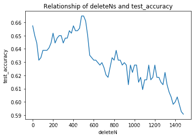
meanaccuracy = pd.DataFrame(accuracy,columns =range(0,1500,20)).mean()#绘图import matplotlib.pyplot as plt
plt.figure()
plt.plot(deleteNs,meanaccuracy)
plt.title('Relationship of deleteNs and test_accuracy')
plt.xlabel('deleteN')
plt.ylabel('test_accuracy')
plt.show()
import numpy as np
meanaccuracy.idxmax()
480
这样就可以确定一定较为合适的deleteN的值
BernoulliNB
BernoulliNB就是先验为伯努利分布的朴素贝叶斯,假设特征的先验概率为二元伯努利分布,即如下式:
(
X
j
=
X
j
l
∣
Y
=
C
k
)
=
P
(
j
∣
Y
=
C
k
)
x
j
l
+
(
1
−
P
(
j
∣
Y
=
C
k
)
)
(
1
−
x
j
l
)
(X_j = X_{jl}|Y=C_k)=P(j|Y=C_k)x_{jl}+(1-P(j|Y=C_k))(1-x_{jl})
(Xj=Xjl∣Y=Ck)=P(j∣Y=Ck)xjl+(1−P(j∣Y=Ck))(1−xjl) 此时l只有两种取值,即x_{jl}只能取0或者1 在伯努利模型中,每个特征的取值是布尔型,即true和false,在文本分类中,就只一个特征有没有在一个文档中出现。