特征工程，使用线性回归机制来拟合非常复杂甚至非线性(存在 x n x^n xn)的函数。

1. 导入

import numpy as np
import matplotlib.pyplot as plt
from lab_utils_multi import zscore_normalize_features, run_gradient_descent_feng
np.set_printoptions(precision=2)  # reduced display precision on numpy arrays

2.多项式特征

这是线性回归时使用的
f w , b = w 0 x 0 + w 1 x 1 + . . . + w n − 1 x n − 1 + b (1) f_{\mathbf{w},b} = w_0x_0 + w_1x_1+ ... + w_{n-1}x_{n-1} + b \tag{1} fw,b​=w0​x0​+w1​x1​+...+wn−1​xn−1​+b(1)

先看看按照以前的线性回归方法的效果

# create target data
x = np.arange(0, 20, 1)
y = 1 + x**2
X = x.reshape(-1, 1)

model_w,model_b = run_gradient_descent_feng(X,y,iterations=1000, alpha = 1e-2)

plt.scatter(x, y, marker='x', c='r', label="Actual Value"); plt.title("no feature engineering")
plt.plot(x,X@model_w + model_b, label="Predicted Value");  plt.xlabel("X"); plt.ylabel("y"); plt.legend(); plt.show()

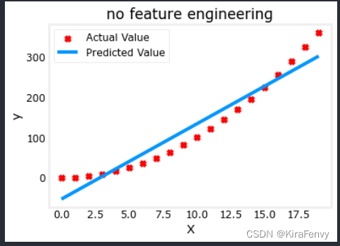
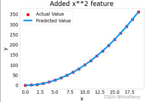
明显不行，我们需要多项式特征，因此我们进行特征工程，调整x的次数

# create target data
x = np.arange(0, 20, 1)
y = 1 + x**2

# Engineer features 
X = x**2      #<-- added engineered feature

X = X.reshape(-1, 1)  #X should be a 2-D Matrix
model_w,model_b = run_gradient_descent_feng(X, y, iterations=10000, alpha = 1e-5)

Iteration         0, Cost: 7.32922e+03
Iteration      1000, Cost: 2.24844e-01
Iteration      2000, Cost: 2.22795e-01
Iteration         0, Cost: 7.32922e+03
Iteration      1000, Cost: 2.24844e-01
Iteration      2000, Cost: 2.22795e-01
Iteration      3000, Cost: 2.20764e-01
Iteration      4000, Cost: 2.18752e-01
Iteration      5000, Cost: 2.16758e-01
Iteration      3000, Cost: 2.20764e-01
Iteration      4000, Cost: 2.18752e-01
Iteration      5000, Cost: 2.16758e-01
Iteration      6000, Cost: 2.14782e-01
Iteration      7000, Cost: 2.12824e-01
Iteration      8000, Cost: 2.10884e-01
Iteration      6000, Cost: 2.14782e-01
Iteration      7000, Cost: 2.12824e-01
Iteration      8000, Cost: 2.10884e-01
Iteration      9000, Cost: 2.08962e-01
w,b found by gradient descent: w: [1.], b: 0.0490
Iteration      9000, Cost: 2.08962e-01
w,b found by gradient descent: w: [1.], b: 0.0490


plt.scatter(x, y, marker='x', c='r', label="Actual Value"); plt.title("Added x**2 feature")
plt.plot(x, np.dot(X,model_w) + model_b, label="Predicted Value"); plt.xlabel("x"); plt.ylabel("y"); plt.legend(); plt.show()

拟合出来的式子是 y = 1 ∗ x 0 2 + 0.049 y=1*x_0^2+0.049 y=1∗x02​+0.049

3.特征选择

Above, we knew that an x 2 x^2 x2 term was required. It may not always be obvious which features are required. One could add a variety of potential features to try and find the most useful. For example, what if we had instead tried : y = w 0 x 0 + w 1 x 1 2 + w 2 x 2 3 + b y=w_0x_0 + w_1x_1^2 + w_2x_2^3+b y=w0​x0​+w1​x12​+w2​x23​+b ?
试一下别的，看拟合程度会不会更高

# create target data
x = np.arange(0, 20, 1)
y = x**2

# engineer features .
X = np.c_[x, x**2, x**3]   #<-- added engineered feature

model_w,model_b = run_gradient_descent_feng(X, y, iterations=10000, alpha=1e-7)

plt.scatter(x, y, marker='x', c='r', label="Actual Value"); plt.title("x, x**2, x**3 features")
plt.plot(x, X@model_w + model_b, label="Predicted Value"); plt.xlabel("x"); plt.ylabel("y"); plt.legend(); plt.show()


Iteration         0, Cost: 1.14029e+03
Iteration      1000, Cost: 3.28539e+02
Iteration      2000, Cost: 2.80443e+02
Iteration         0, Cost: 1.14029e+03
Iteration      1000, Cost: 3.28539e+02
Iteration      2000, Cost: 2.80443e+02
Iteration      3000, Cost: 2.39389e+02
Iteration      4000, Cost: 2.04344e+02
Iteration      5000, Cost: 1.74430e+02
Iteration      3000, Cost: 2.39389e+02
Iteration      4000, Cost: 2.04344e+02
Iteration      5000, Cost: 1.74430e+02
Iteration      6000, Cost: 1.48896e+02
Iteration      7000, Cost: 1.27100e+02
Iteration      8000, Cost: 1.08495e+02
Iteration      6000, Cost: 1.48896e+02
Iteration      7000, Cost: 1.27100e+02
Iteration      8000, Cost: 1.08495e+02
Iteration      9000, Cost: 9.26132e+01
w,b found by gradient descent: w: [0.08 0.54 0.03], b: 0.0106

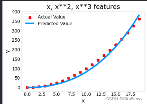
拟合出来的式子： 0.08 x + 0.54 x 2 + 0.03 x 3 + 0.0106 0.08x + 0.54x^2 + 0.03x^3 + 0.0106 0.08x+0.54x2+0.03x3+0.0106

梯度下降通过强调其相关参数为我们选择“正确”的特征，较小的权重值意味着不太重要/正确的特征

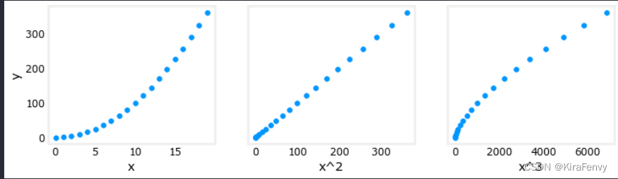
4.多项式特征与线性特征的关联

我们进行多项式回归，也是在选择和y线性关联程度最高的特征

# create target data
x = np.arange(0, 20, 1)
y = x**2

# engineer features .
X = np.c_[x, x**2, x**3]   #<-- added engineered feature
X_features = ['x','x^2','x^3']

fig,ax=plt.subplots(1, 3, figsize=(12, 3), sharey=True)
for i in range(len(ax)):
    ax[i].scatter(X[:,i],y)
    ax[i].set_xlabel(X_features[i])
ax[0].set_ylabel("y")
plt.show()

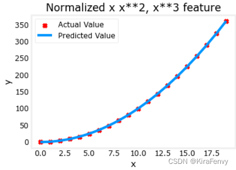
5. 特征缩放 Scaling features

# create target data
x = np.arange(0,20,1)
X = np.c_[x, x**2, x**3]
print(f"Peak to Peak range by column in Raw        X:{np.ptp(X,axis=0)}")

# add mean_normalization 
X = zscore_normalize_features(X)     
print(f"Peak to Peak range by column in Normalized X:{np.ptp(X,axis=0)}")

Peak to Peak range by column in Raw        X:[  19  361 6859]
Peak to Peak range by column in Normalized X:[3.3  3.18 3.28]
Peak to Peak range by column in Raw        X:[  19  361 6859]
Peak to Peak range by column in Normalized X:[3.3  3.18 3.28]

x = np.arange(0,20,1)
y = x**2

X = np.c_[x, x**2, x**3]
X = zscore_normalize_features(X) 

model_w, model_b = run_gradient_descent_feng(X, y, iterations=100000, alpha=1e-1)

plt.scatter(x, y, marker='x', c='r', label="Actual Value"); plt.title("Normalized x x**2, x**3 feature")
plt.plot(x,X@model_w + model_b, label="Predicted Value"); plt.xlabel("x"); plt.ylabel("y"); plt.legend(); plt.show()

Iteration         0, Cost: 9.42147e+03
Iteration         0, Cost: 9.42147e+03
Iteration     10000, Cost: 3.90938e-01
Iteration     10000, Cost: 3.90938e-01
Iteration     20000, Cost: 2.78389e-02
Iteration     20000, Cost: 2.78389e-02
Iteration     30000, Cost: 1.98242e-03
Iteration     30000, Cost: 1.98242e-03
Iteration     40000, Cost: 1.41169e-04
Iteration     40000, Cost: 1.41169e-04
Iteration     50000, Cost: 1.00527e-05
Iteration     50000, Cost: 1.00527e-05
Iteration     60000, Cost: 7.15855e-07
Iteration     60000, Cost: 7.15855e-07
Iteration     70000, Cost: 5.09763e-08
Iteration     70000, Cost: 5.09763e-08
Iteration     80000, Cost: 3.63004e-09
Iteration     80000, Cost: 3.63004e-09
Iteration     90000, Cost: 2.58497e-10
Iteration     90000, Cost: 2.58497e-10
w,b found by gradient descent: w: [5.27e-05 1.13e+02 8.43e-05], b: 123.5000
w,b found by gradient descent: w: [5.27e-05 1.13e+02 8.43e-05], b: 123.5000

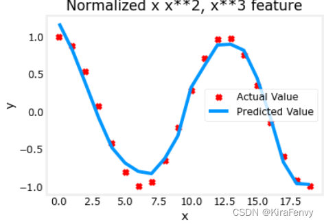
6.复杂函数的拟合

x = np.arange(0,20,1)
y = np.cos(x/2)

X = np.c_[x, x**2, x**3,x**4, x**5, x**6, x**7, x**8, x**9, x**10, x**11, x**12, x**13]
X = zscore_normalize_features(X) 

model_w,model_b = run_gradient_descent_feng(X, y, iterations=1000000, alpha = 1e-1)

plt.scatter(x, y, marker='x', c='r', label="Actual Value"); plt.title("Normalized x x**2, x**3 feature")
plt.plot(x,X@model_w + model_b, label="Predicted Value"); plt.xlabel("x"); plt.ylabel("y"); plt.legend(); plt.show()

Iteration         0, Cost: 2.24887e-01
Iteration         0, Cost: 2.24887e-01
Iteration    100000, Cost: 2.31061e-02
Iteration    100000, Cost: 2.31061e-02
Iteration    200000, Cost: 1.83619e-02
Iteration    200000, Cost: 1.83619e-02
Iteration    300000, Cost: 1.47950e-02
Iteration    300000, Cost: 1.47950e-02
Iteration    400000, Cost: 1.21114e-02
Iteration    400000, Cost: 1.21114e-02
Iteration    500000, Cost: 1.00914e-02
Iteration    500000, Cost: 1.00914e-02
Iteration    600000, Cost: 8.57025e-03
Iteration    600000, Cost: 8.57025e-03
Iteration    700000, Cost: 7.42385e-03
Iteration    700000, Cost: 7.42385e-03
Iteration    800000, Cost: 6.55908e-03
Iteration    800000, Cost: 6.55908e-03
Iteration    900000, Cost: 5.90594e-03
Iteration    900000, Cost: 5.90594e-03
w,b found by gradient descent: w: [-1.61e+00 -1.01e+01  3.00e+01 -6.92e-01 -2.37e+01 -1.51e+01  2.09e+01
 -2.29e-03 -4.69e-03  5.51e-02  1.07e-01 -2.53e-02  6.49e-02], b: -0.0073
w,b found by gradient descent: w: [-1.61e+00 -1.01e+01  3.00e+01 -6.92e-01 -2.37e+01 -1.51e+01  2.09e+01
 -2.29e-03 -4.69e-03  5.51e-02  1.07e-01 -2.53e-02  6.49e-02], b: -0.0073

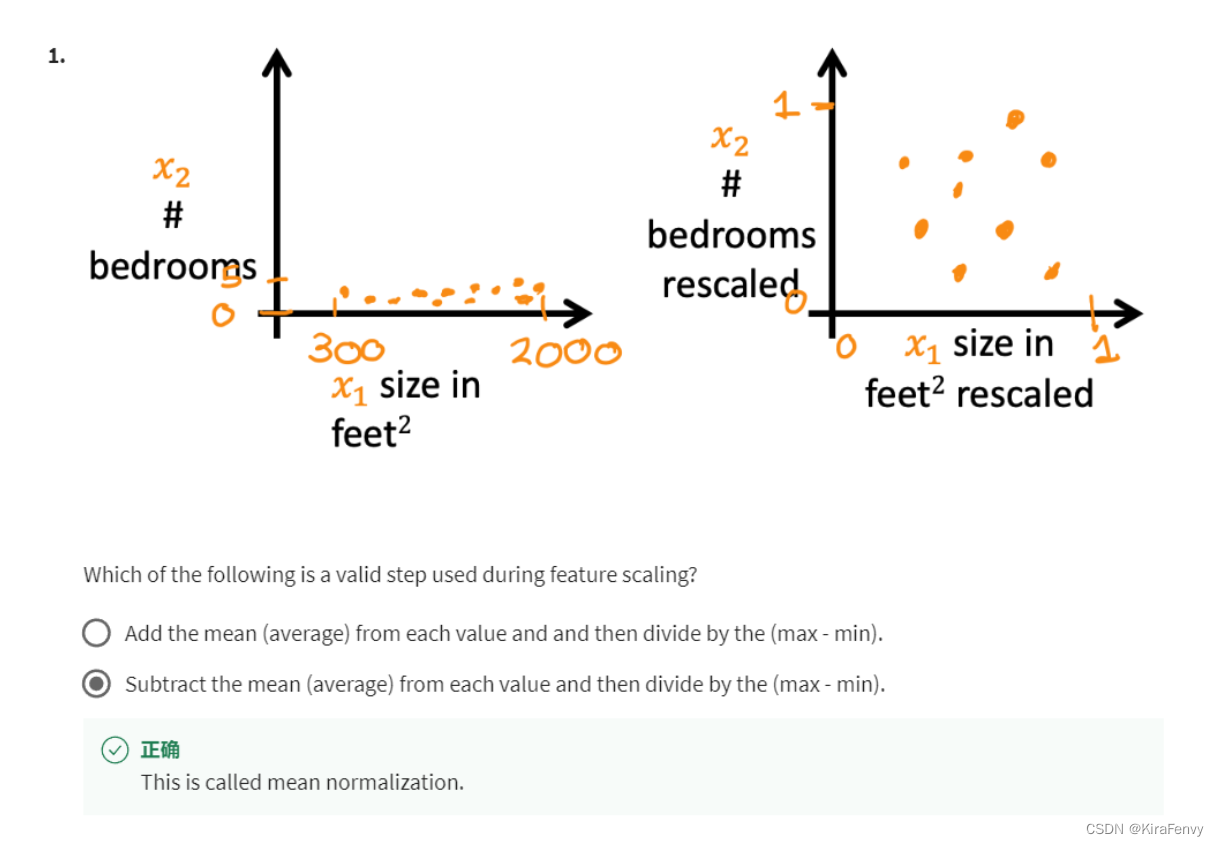
7.课后题

1. 特征缩放的时候要减去平均值
   
2. 代价不能较快的减少证明学习率偏大，代价反而增大证明学习率太大
   
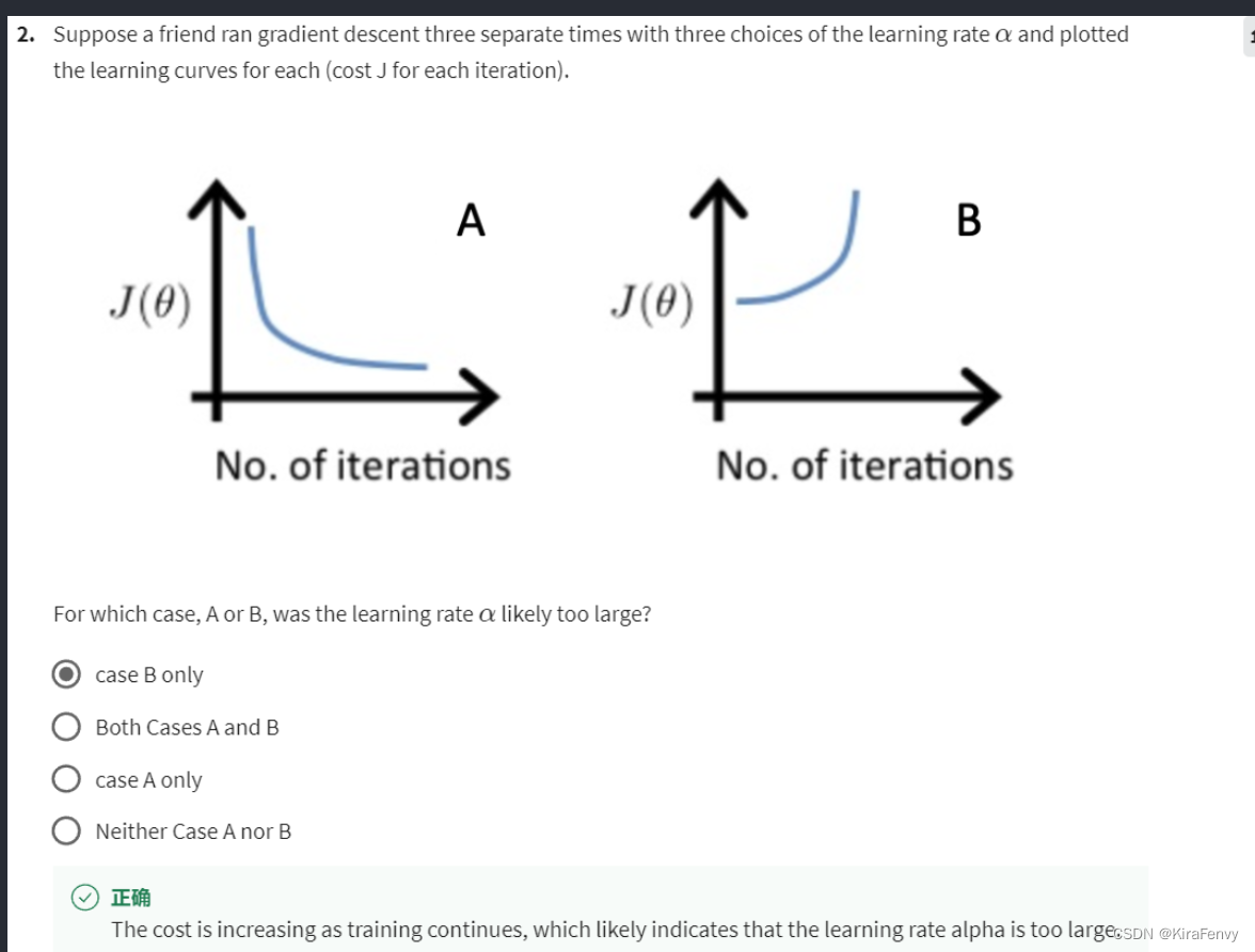
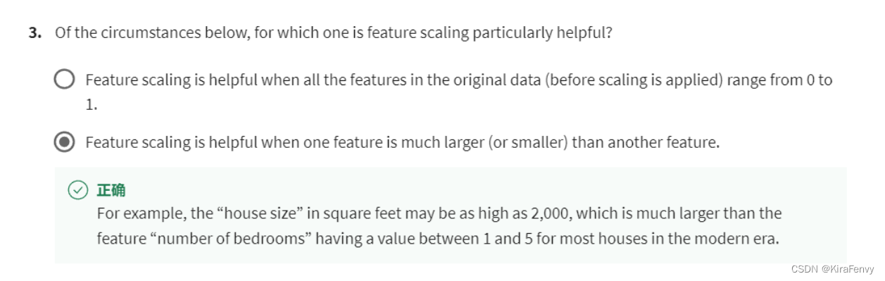
3. 当特征之间的具体数值差距过大的时候，需要用到特征缩放

4. 数量乘价格才是销售总价