seaborn.histplot(data, x, y, hue, stat, bins, bandwidth, discrete, KDE, log_scale)
参数为:
data:输入数据,主要作为数据框 or NumPy 数组.
x, y(可选参数):分别定位在x、y轴上的数据的key
色调(可选参数):映射以确定绘图元素颜色的语义数据键
stat(可选):它测量频率、计数、密度或概率
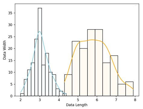
核密度估计(KDE):它是用于平滑直方图的机制之一。
这是一个代码片段:
import seaborn as sns
import numpy as np
import pandas as pd
import matplotlib.pyplot as plt
# Creating arbitrary dataset from random numbers
np.random.seed(1)
numb_var = np.random.randn(1200)
numb_var = pd.Series(numb_var, name = "Numerical Measures")
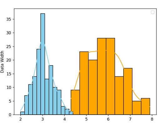
# Plotting the histogram
sns.histplot(data = numb_var, kde=True)
plt.show()
Output
添加标签
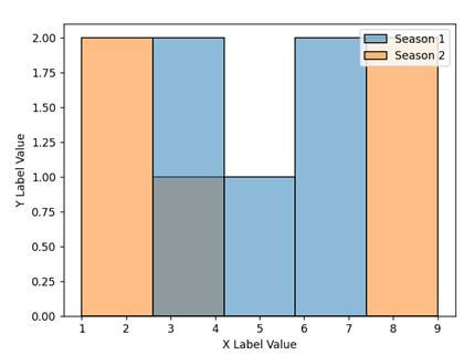
我们经常需要标记 x 轴和 y 轴,以便更好地识别绘图或赋予绘图含义。 Seaborn 提供两种不同的方式来设置 x 轴和 y 轴的标签。 Method 1:使用 set() 方法:set() 方法允许我们设置标签,我们必须在其中传递 xlabel 和 ylabel 参数的字符串。这是一个代码片段,展示了我们如何执行此操作。
import pandas as pd
import matplotlib.pyplot as plt
import seaborn as sns
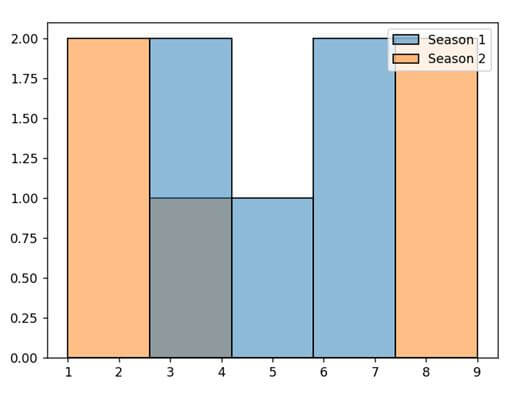
datf = pd.DataFrame({"Season 1": [7, 4, 5, 6, 3],
"Season 2" : [1, 2, 8, 4, 9]})
p = sns.histplot(data = datf)
p.set(xlabel="X Label Value", ylabel = "Y Label Value")
plt.show()
Output
Method 2: Using Matplotlib’s xlabel() and ylabel(): Seaborn runs on top of Matplotlib. Thus, it allows us to leverage Matplotlib pyplot’s xlabel() and ylabel() to create so. The code snippet will look like:
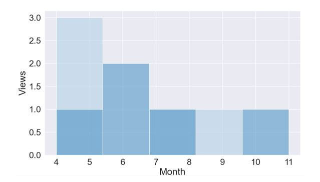
Method 2: Using set_ticklabels() method: This is another method to create empty labels is by using yte xaxis.set_ticklabels() and yaxis.set_ticklabels() and pass an empty list [] as parameter.
import pandas as pd
import matplotlib.pyplot as plt
import seaborn as sns
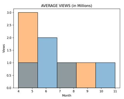
datf = pd.DataFrame({"Season 1": [8, 6, 6, 11, 4],
"Season 2" : [4, 5, 7, 4, 9]})
p = sns.histplot(data = datf).set(title = "AVERAGE VIEWS (in Millions)")
plt.xlabel('Month')
plt.ylabel('Views')
plt.legend([],[], frameon = False)
plt.show()
Output
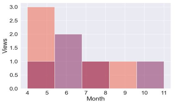
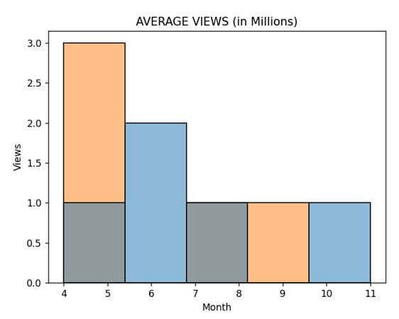
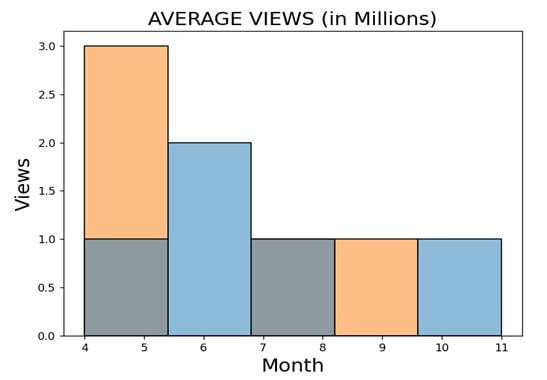
Method 2: Using the set_title() method: This method works as a helping substitute method for string and takes the string as a parameter within the plot. Here is a code snippet on how to use it.
import pandas as pd
import matplotlib.pyplot as plt
import seaborn as sns
datf = pd.DataFrame({"Season 1": [8, 6, 6, 11, 4],
                 "Season 2" : [4, 5, 7, 4, 9]})
p = sns.histplot(data = datf).set_title('AVERAGE VIEWS (in Millions)')
plt.xlabel('Month')
plt.ylabel('Views')
plt.legend([],[], frameon = False)
plt.show()
Output
Method 3: Using Matplotlib’s title() method: Since Seaborn runs on top of Matplotlib, we can efficiently utilize Matplotlib’s title() method to specify the title for the plot. Here is a code snippet showing its use.
import pandas as pd
import matplotlib.pyplot as plt
import seaborn as sns
datf = pd.DataFrame({"Season 1": [8, 6, 6, 11, 4],
                 "Season 2" : [4, 5, 7, 4, 9]})
p = sns.histplot(data = datf)
plt.title("AVERAGE VIEWS (in Millions)")
plt.xlabel('Month')
plt.ylabel('Views')
plt.legend([],[], frameon = False)
plt.show()
Method 2: Using the set() method: The set() method also helps to set up the font size for all the fonts related to the plot and font_scale parameter. Here’s how to use it.
import pandas as pd
import matplotlib.pyplot as plt
import seaborn as sns
datf = pd.DataFrame({"Season 1": [8, 6, 6, 11, 4],
                 "Season 2" : [4, 5, 7, 4, 9]})
sns.set(font_scale = 3)
p = sns.histplot(data = datf)
p.set_xlabel("Month")
p.set_ylabel("Views")
p.set_title("AVERAGE VIEWS (in Millions)")
plt.legend([],[], frameon = False)
plt.show()
import matplotlib.pyplot as plt
import seaborn as sns
tips = sns.load_dataset("tips")
tips.head()
#Changing the orientation of the plot
g = sns.histplot(data=tips, y="total_bill", color="lime")
g.set_ylabel("Bill", fontsize=12)
g.set_xlabel("")
plt.show()
 Or,
Or,