3 EKF SLAM
在上一节中我们看到的是扩展卡尔曼滤波在定位中的应用,EKF同样可以应用于SLAM问题中。在定位问题中,机器人接收到的观测值是其在二维空间中的x-y位置。如果机器人接收到的是跟周围环境有关的信息,例如机器人某时刻下距离某路标点的距离和角度,那么我们可以根据此时机器人自身位置的估计值,推测出该路标点在二维空间中的位置,将路标点的空间位置也作为待修正的状态量放入整个的状态向量中。
由此又引出了两个子问题:数据关联和状态扩增。
我们将通过以下python实例来理解ekf slam的原理(完整代码见原链接,有中文注释的附在了最后):

- 黑色星号: 路标点真实位置(代码中RFID数组代表真实位置)
- 绿色×: 路标点位置估计值
- 黑色线: 航迹推测方法得出的机器人轨迹
- 蓝色线: 轨迹真值
- 红色线: EKF SLAM得出的机器人轨迹
回想上一节的扩展卡尔曼滤波的公式:
=== Predict ===
x
P
r
e
d
=
F
x
t
+
B
u
t
x_{Pred} = Fx_t+Bu_t
xPred=Fxt+But
P
P
r
e
d
=
J
F
P
t
J
F
T
+
Q
P_{Pred} = J_FP_t J_F^T + Q
PPred=JFPtJFT+Q
=== Update ===
z
P
r
e
d
=
H
x
P
r
e
d
z_{Pred} = Hx_{Pred}
zPred=HxPred
y
=
z
−
z
P
r
e
d
y = z - z_{Pred}
y=z−zPred
S
=
J
H
P
P
r
e
d
.
J
H
T
+
R
S = J_H P_{Pred}.J_H^T + R
S=JHPPred.JHT+R
K
=
P
P
r
e
d
.
J
H
T
S
−
1
K = P_{Pred}.J_H^T S^{-1}
K=PPred.JHTS−1
x
t
+
1
=
x
P
r
e
d
+
K
y
x_{t+1} = x_{Pred} + Ky
xt+1=xPred+Ky
P
t
+
1
=
(
I
−
K
J
H
)
P
P
r
e
d
P_{t+1} = ( I - K J_H) P_{Pred}
Pt+1=(I−KJH)PPred
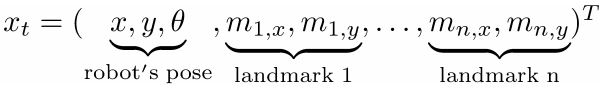
EKF SLAM 使用一个EKF滤波器来解决SLAM问题,EKF SLAM的状态向量包括了机器人位姿
(
x
,
y
,
θ
)
(x, y, \theta)
(x,y,θ) 和观测到的各个路标点的坐标
[
(
m
1
x
,
m
1
y
)
,
(
m
2
x
,
m
2
y
)
,
.
.
.
,
(
m
n
x
,
m
n
y
)
]
[(m_1x, m_1y), (m_2x, m_2y), ... , (m_nx, m_ny)]
[(m1x,m1y),(m2x,m2y),...,(mnx,mny)] ,路标点与机器人位姿间的协方差矩阵也在更新。
相应的协方差矩阵:

可以简写作:

需要注意的是,由于状态向量中包含路标点位置坐标,所以随着机器人运动,观测到的路标点会越来越多,因此状态向量和状态协方差矩阵会不断变化。
运动模型
状态向量预测 在状态向量中,只有机器人位姿状态
(
x
,
y
,
θ
)
(x, y, \theta)
(x,y,θ)是随着机器人运动改变的,所以运动模型影响下的状态向量预测这步中只改变状态向量中的这三个值和协方差矩阵中对应的区域。以下是本实例中使用的运动模型,控制输入向量为机器人线速度和角速度
(
v
,
w
)
(v,w)
(v,w)。
F
=
[
1
0
0
0
1
0
0
0
1
]
\begin{aligned} F= \begin{bmatrix} 1 & 0 & 0 \\ 0 & 1 & 0 \\ 0 & 0 & 1 \end{bmatrix} \end{aligned}
F=⎣⎡100010001⎦⎤
B
=
[
Δ
t
c
o
s
(
θ
)
0
Δ
t
s
i
n
(
θ
)
0
0
Δ
t
]
\begin{aligned} B= \begin{bmatrix} \Delta t cos(\theta) & 0\\ \Delta t sin(\theta) & 0\\ 0 & \Delta t \end{bmatrix} \end{aligned}
B=⎣⎡Δtcos(θ)Δtsin(θ)000Δt⎦⎤
U
=
[
v
t
w
t
]
\begin{aligned} U= \begin{bmatrix} v_t\\ w_t\\ \end{bmatrix} \end{aligned}
U=[vtwt]
X
=
F
X
+
B
U
\begin{aligned} X = FX + BU \end{aligned}
X=FX+BU
[
x
t
+
1
y
t
+
1
θ
t
+
1
]
=
[
1
0
0
0
1
0
0
0
1
]
[
x
t
y
t
θ
t
]
+
[
Δ
t
c
o
s
(
θ
)
0
Δ
t
s
i
n
(
θ
)
0
0
Δ
t
]
[
v
t
+
σ
v
w
t
+
σ
w
]
\begin{aligned} \begin{bmatrix} x_{t+1} \\ y_{t+1} \\ \theta_{t+1} \end{bmatrix}= \begin{bmatrix} 1 & 0 & 0 \\ 0 & 1 & 0 \\ 0 & 0 & 1 \end{bmatrix}\begin{bmatrix} x_{t} \\ y_{t} \\ \theta_{t} \end{bmatrix}+ \begin{bmatrix} \Delta t cos(\theta) & 0\\ \Delta t sin(\theta) & 0\\ 0 & \Delta t \end{bmatrix} \begin{bmatrix} v_{t} + \sigma_v\\ w_{t} + \sigma_w\\ \end{bmatrix} \end{aligned}
⎣⎡xt+1yt+1θt+1⎦⎤=⎣⎡100010001⎦⎤⎣⎡xtytθt⎦⎤+⎣⎡Δtcos(θ)Δtsin(θ)000Δt⎦⎤[vt+σvwt+σw]
可以看出运动模型与上一节中的并无不同(只是状态向量有区别),
U
U
U 是包含线速度角速度
v
t
v_t
vt 和
w
t
w_t
wt的控制输入向量,
+
σ
v
+\sigma_v
+σv 和
+
σ
w
+\sigma_w
+σw 表示控制输入也包含噪声。
协方差预测 对机器人位姿状态的协方差进行预测,本质上是加上运动模型误差,位姿的不确定性通过加上运动模型的协方差
Q
Q
Q而增加了。
P
=
G
T
P
G
+
Q
P = G^TPG + Q
P=GTPG+Q
注意:这里的
G
G
G就是上一节公式中的雅克比矩阵
J
F
J_F
JF,为与python代码保持一致,这里不再改动。
在这一步骤中,协方差矩阵
P
P
P里只有与机器人位姿相关的部分被修改,与路标点相关的部分没有改动。
def motion_model(x, u):
"""
根据控制预测机器人位姿
"""
F = np.array([[1.0, 0, 0],
[0, 1.0, 0],
[0, 0, 1.0]])
B = np.array([[DT * math.cos(x[2, 0]), 0],
[DT * math.sin(x[2, 0]), 0],
[0.0, DT]])
x = (F @ x) + (B @ u)
return x
def jacob_motion(x, u):
Fx = np.hstack((np.eye(STATE_SIZE), np.zeros(
(STATE_SIZE, LM_SIZE * calc_n_lm(x)))))
jF = np.array([[0.0, 0.0, -DT * u[0] * math.sin(x[2, 0])],
[0.0, 0.0, DT * u[0] * math.cos(x[2, 0])],
[0.0, 0.0, 0.0]], dtype=np.float64)
G = np.eye(STATE_SIZE) + Fx.T @ jF @ Fx
return G, Fx,
观测模型
在这个实例中,观测模型比上一节要复杂,因为实例模拟的是激光雷达检测路标点获得的与机器人距离和角度的信息。观测值向量
z
z
z包含的两个元素就是机器人与路标点的相对距离和角度,因此单个路标点在二维空间内的坐标就可以通过机器人在二维空间内的坐标得出:

等式左边就是第j个路标点在二维空间内的坐标。
相应地,可以得到机器人位姿状态与单个路标点观测值之间的转换关系,也就是观测模型:

所以单个路标点的雅克比矩阵表示为:
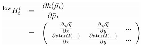
(说明:
H
t
H_t
Ht矩阵左上角的low表示这是针对单个路标点的雅克比矩阵,右上角的i表示这是对应第i组观测值的雅克比矩阵)
对于每个路标点,观测雅克比矩阵需要进行偏微分的有以下5个元素:
(
μ
‾
t
,
x
,
μ
‾
t
,
y
,
μ
‾
t
,
θ
,
μ
‾
j
,
x
,
μ
‾
j
,
y
)
(\overline\mu_{t,x}, \overline\mu_{t,y}, \overline\mu_{t,\theta}, \overline\mu_{j,x},\overline\mu_{j,y})
(μt,x,μt,y,μt,θ,μj,x,μj,y)
分别是机器人位姿状态和该路标点的二维x-y空间位置。
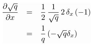
推导可得:
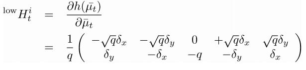
单个路标点的雅克比矩阵作用于整个观测模型雅克比矩阵上需要乘以一个矩阵
F
x
,
j
F_{x,j}
Fx,j,来把单个雅克比矩阵的元素放到对应位置上,j就表示是第几个路标点。
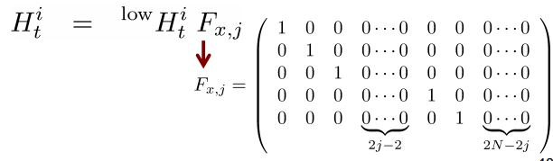
2
j
−
2
=
2
(
j
−
1
)
2j-2=2(j-1)
2j−2=2(j−1)表示第j个路标点前的j-1个路标点的位置,
2
N
−
2
j
=
2
(
N
−
j
)
2N-2j=2(N-j)
2N−2j=2(N−j)表示第j个路标点之后的N-j个路标点(N在此表示一共有N个路标点)的位置,这些位置都是0,因为该路标点不会作用于其他路标点。
def calc_innovation(lm, xEst, PEst, z, LMid):
"""
Calculates the innovation based on expected position and landmark position
:param lm: landmark position
:param xEst: estimated position/state
:param PEst: estimated covariance
:param z: read measurements
:param LMid: landmark id
:returns: returns the innovation y, and the jacobian H, and S, used to calculate the Kalman Gain
"""
delta = lm - xEst[0:2]
q = (delta.T @ delta)[0, 0]
z_angle = math.atan2(delta[1, 0], delta[0, 0]) - xEst[2, 0]
zp = np.array([[math.sqrt(q), pi_2_pi(z_angle)]])
y = (z - zp).T
y[1] = pi_2_pi(y[1])
H = jacob_h(q, delta, xEst, LMid + 1)
S = H @ PEst @ H.T + R
return y, S, H
def jacob_h(q, delta, x, i):
"""
Calculates the jacobian of the measurement function
:param q: the range from the system pose to the landmark
:param delta: the difference between a landmark position and the estimated system position
:param x: the state, including the estimated system position
:param i: landmark id + 1
:returns: the jacobian H
"""
sq = math.sqrt(q)
G = np.array([[-sq * delta[0, 0], - sq * delta[1, 0], 0, sq * delta[0, 0], sq * delta[1, 0]],
[delta[1, 0], - delta[0, 0], - q, - delta[1, 0], delta[0, 0]]])
G = G / q
nLM = calc_n_lm(x)
F1 = np.hstack((np.eye(3), np.zeros((3, 2 * nLM))))
F2 = np.hstack((np.zeros((2, 3)), np.zeros((2, 2 * (i - 1))),
                    np.eye(2), np.zeros((2, 2 * nLM - 2 * i))))
F = np.vstack((F1, F2))
H = G @ F
return H
其中jacob_h函数中的这几行代码:
F1 = np.hstack((np.eye(3), np.zeros((3, 2 * nLM))))
F2 = np.hstack((np.zeros((2, 3)), np.zeros((2, 2 * (i - 1))),
np.eye(2), np.zeros((2, 2 * nLM - 2 * i))))
F = np.vstack((F1, F2))
就是在构建上面推导的算式中的
F
x
,
j
F_{x,j}
Fx,j矩阵,在代码中,nLM表示路标点总数,i表示路标点的id,运行几个例子来看看
F
x
,
j
F_{x,j}
Fx,j矩阵的细节:
import numpy as np
nLM = 3
i = 1
F1 = np.hstack((np.eye(3), np.zeros((3, 2 * nLM))))
F2 = np.hstack((np.zeros((2, 3)), np.zeros((2, 2 * (i - 1))),np.eye(2), np.zeros((2, 2 * nLM - 2 * i))))
F = np.vstack((F1, F2))
print(F1)
print(F2)
print(F)
[[ 1.  0.  0.  0.  0.  0.  0.  0.  0.]
 [ 0.  1.  0.  0.  0.  0.  0.  0.  0.]
 [ 0.  0.  1.  0.  0.  0.  0.  0.  0.]]
[[ 0.  0.  0.  1.  0.  0.  0.  0.  0.]
 [ 0.  0.  0.  0.  1.  0.  0.  0.  0.]]
[[ 1.  0.  0.  0.  0.  0.  0.  0.  0.]
 [ 0.  1.  0.  0.  0.  0.  0.  0.  0.]
 [ 0.  0.  1.  0.  0.  0.  0.  0.  0.]
 [ 0.  0.  0.  1.  0.  0.  0.  0.  0.]
 [ 0.  0.  0.  0.  1.  0.  0.  0.  0.]]
i = 2
F1 = np.hstack((np.eye(3), np.zeros((3, 2 * nLM))))
F2 = np.hstack((np.zeros((2, 3)), np.zeros((2, 2 * (i - 1))),np.eye(2), np.zeros((2, 2 * nLM - 2 * i))))
F = np.vstack((F1, F2))
print(F1)
print(F2)
print(F)
[[ 1.  0.  0.  0.  0.  0.  0.  0.  0.]
 [ 0.  1.  0.  0.  0.  0.  0.  0.  0.]
 [ 0.  0.  1.  0.  0.  0.  0.  0.  0.]]
[[ 0.  0.  0.  0.  0.  1.  0.  0.  0.]
 [ 0.  0.  0.  0.  0.  0.  1.  0.  0.]]
[[ 1.  0.  0.  0.  0.  0.  0.  0.  0.]
 [ 0.  1.  0.  0.  0.  0.  0.  0.  0.]
 [ 0.  0.  1.  0.  0.  0.  0.  0.  0.]
 [ 0.  0.  0.  0.  0.  1.  0.  0.  0.]
 [ 0.  0.  0.  0.  0.  0.  1.  0.  0.]]
i = 3
F1 = np.hstack((np.eye(3), np.zeros((3, 2 * nLM))))
F2 = np.hstack((np.zeros((2, 3)), np.zeros((2, 2 * (i - 1))),np.eye(2), np.zeros((2, 2 * nLM - 2 * i))))
F = np.vstack((F1, F2))
print(F1)
print(F2)
print(F)
[[ 1.  0.  0.  0.  0.  0.  0.  0.  0.]
 [ 0.  1.  0.  0.  0.  0.  0.  0.  0.]
 [ 0.  0.  1.  0.  0.  0.  0.  0.  0.]]
[[ 0.  0.  0.  0.  0.  0.  0.  1.  0.]
 [ 0.  0.  0.  0.  0.  0.  0.  0.  1.]]
[[ 1.  0.  0.  0.  0.  0.  0.  0.  0.]
 [ 0.  1.  0.  0.  0.  0.  0.  0.  0.]
 [ 0.  0.  1.  0.  0.  0.  0.  0.  0.]
 [ 0.  0.  0.  0.  0.  0.  0.  1.  0.]
 [ 0.  0.  0.  0.  0.  0.  0.  0.  1.]]
在实例中,机器人在每个时刻t都会得到若干组观测值,就像在现实中,每隔一定时间,机器人都会得到传感器的一系列测量值一样。那么如何知道一组观测值
z
t
i
=
(
r
t
i
,
ϕ
t
i
)
T
z_t^i=(r_t^i,\phi_t^i)^T
zti=(rti,ϕti)T 对应的是第几个路标点呢?也就是说,上面第j个路标点的j是怎么得到的?下面简述本python实例中的方案:
对于每一组观测值
z
t
i
=
(
r
t
i
,
ϕ
t
i
)
T
z_t^i=(r_t^i,\phi_t^i)^T
zti=(rti,ϕti)T,计算对应此时刻的机器人位姿,已有的状态向量:

中的从landmark 1到landmark n的每一个路标点的观测值,也就是从此时刻机器人的位置向四周看去,landmark 1到landmark n的观测值,计算这些观测值与观测值
z
t
i
=
(
r
t
i
,
ϕ
t
i
)
T
z_t^i=(r_t^i,\phi_t^i)^T
zti=(rti,ϕti)T的残差,如果这些残差的马哈拉诺比斯距离均大于某一个阈值,则判定这是一个没观测过的新的路标点;如果这些距离不是都大于某个阈值,则我们简单地认为距离最短的那个路标点landmark就是观测值
z
t
i
=
(
r
t
i
,
ϕ
t
i
)
T
z_t^i=(r_t^i,\phi_t^i)^T
zti=(rti,ϕti)T对应的路标点。简单来说,找跟观测值
z
t
i
=
(
r
t
i
,
ϕ
t
i
)
T
z_t^i=(r_t^i,\phi_t^i)^T
zti=(rti,ϕti)T差别最小的那个路标点,如果差别都挺大,那就认为看到了个新的路标点。
马哈拉诺比斯距离的阈值在代码中的值为2.0:
M_DIST_TH = 2.0
在实例中寻找匹配的路标点编号id的对应代码是:
def search_correspond_landmark_id(xAug, PAug, zi):
"""
Landmark association with Mahalanobis distance
"""
nLM = calc_n_lm(xAug)
min_dist = []
for i in range(nLM):
lm = get_landmark_position_from_state(xAug, i)
y, S, H = calc_innovation(lm, xAug, PAug, zi, i)
min_dist.append(y.T @ np.linalg.inv(S) @ y)
min_dist.append(M_DIST_TH)
min_id = min_dist.index(min(min_dist))
return min_id
这种根据残差的马哈拉诺比斯距离最小来寻找匹配的路标点只是一种理想化的简单处理方式,实际应用中的“data association”会复杂得多。
接下来还有一步需要注意,如果
z
t
i
=
(
r
t
i
,
ϕ
t
i
)
T
z_t^i=(r_t^i,\phi_t^i)^T
zti=(rti,ϕti)T是一个未观测过的路标点的观测值,那么需要对状态向量和状态协方差矩阵进行扩增,对应的python代码为:
xAug = np.vstack((xEst, calc_landmark_position(xEst, z[iz, :])))
PAug = np.vstack((np.hstack((PEst, np.zeros((len(xEst), LM_SIZE)))),
np.hstack((np.zeros((LM_SIZE, len(xEst))), initP))))
xEst = xAug
PEst = PAug
其中的initP是一个对角元素为1的2×2矩阵,代表给新增的一个路标点的状态量协方差一个初始值。
至此,我们了解了机器人对路标点的观测模型,以及如何计算观测模型的雅克比矩阵,接下来就可以继续计算卡尔曼增益
K
K
K,执行EKF中的更新步骤了。整个更新步骤的算法总结如下:


最后再说一点此实例中有关仿真数据生成的内容,在observation函数中,根据机器人位姿真值决定机器人可以看到哪几个路标点,再将这几个路标点的观测值人为加上噪声。
参考链接:
SLAM笔记五——EKF-SLAM
PythonRobotics/SLAM/EKFSLAM
附上带中文注释的完整代码:
"""
Extended Kalman Filter SLAM example
author: Atsushi Sakai (@Atsushi_twi)
https://github.com/AtsushiSakai/PythonRobotics/tree/master/SLAM/EKFSLAM
"""
import math
import matplotlib.pyplot as plt
import numpy as np
Q = np.diag([0.5, 0.5, np.deg2rad(30.0)]) ** 2
R = np.diag([0.5, 0.5])**2
Q_sim = np.diag([0.2, np.deg2rad(1.0)]) ** 2
R_sim = np.diag([1.0, np.deg2rad(10.0)]) ** 2
DT = 0.1
SIM_TIME = 50.0
MAX_RANGE = 20.0
M_DIST_TH = 2.0
STATE_SIZE = 3
LM_SIZE = 2
show_animation = True
def ekf_slam(xEst, PEst, u, z):
S = STATE_SIZE
G, Fx = jacob_motion(xEst[0:S], u)
xEst[0:S] = motion_model(xEst[0:S], u)
PEst[0:S, 0:S] = G.T @ PEst[0:S, 0:S] @ G + Fx.T @ Q @ Fx
initP = np.eye(2)
for iz in range(len(z[:, 0])):
min_id = search_correspond_landmark_id(xEst, PEst, z[iz, 0:2])
nLM = calc_n_lm(xEst)
if min_id == nLM:
print("New LM")
xAug = np.vstack((xEst, calc_landmark_position(xEst, z[iz, :])))
PAug = np.vstack((np.hstack((PEst, np.zeros((len(xEst), LM_SIZE)))),
np.hstack((np.zeros((LM_SIZE, len(xEst))), initP))))
xEst = xAug
PEst = PAug
lm = get_landmark_position_from_state(xEst, min_id)
y, S, H = calc_innovation(lm, xEst, PEst, z[iz, 0:2], min_id)
K = (PEst @ H.T) @ np.linalg.inv(S)
xEst = xEst + (K @ y)
PEst = (np.eye(len(xEst)) - (K @ H)) @ PEst
xEst[2] = pi_2_pi(xEst[2])
return xEst, PEst
def calc_input():
v = 1.0
yaw_rate = 0.1
u = np.array([[v, yaw_rate]]).T
return u
def observation(xTrue, xd, u, RFID):
"""
仿真过程
"""
xTrue = motion_model(xTrue, u)
z = np.zeros((0, 3))
for i in range(len(RFID[:, 0])):
dx = RFID[i, 0] - xTrue[0, 0]
dy = RFID[i, 1] - xTrue[1, 0]
d = math.hypot(dx, dy)
angle = pi_2_pi(math.atan2(dy, dx) - xTrue[2, 0])
if d <= MAX_RANGE:
dn = d + np.random.randn() * Q_sim[0, 0] ** 0.5
angle_n = angle + np.random.randn() * Q_sim[1, 1] ** 0.5
zi = np.array([dn, angle_n, i])
z = np.vstack((z, zi))
ud = np.array([[
u[0, 0] + np.random.randn() * R_sim[0, 0] ** 0.5,
u[1, 0] + np.random.randn() * R_sim[1, 1] ** 0.5]]).T
xd = motion_model(xd, ud)
return xTrue, z, xd, ud
def motion_model(x, u):
"""
根据控制预测机器人位姿
"""
F = np.array([[1.0, 0, 0],
[0, 1.0, 0],
[0, 0, 1.0]])
B = np.array([[DT * math.cos(x[2, 0]), 0],
[DT * math.sin(x[2, 0]), 0],
[0.0, DT]])
x = (F @ x) + (B @ u)
return x
def calc_n_lm(x):
"""
返回Landmark的个数
"""
n = int((len(x) - STATE_SIZE) / LM_SIZE)
return n
def jacob_motion(x, u):
Fx = np.hstack((np.eye(STATE_SIZE), np.zeros(
(STATE_SIZE, LM_SIZE * calc_n_lm(x)))))
jF = np.array([[0.0, 0.0, -DT * u[0] * math.sin(x[2, 0])],
[0.0, 0.0, DT * u[0] * math.cos(x[2, 0])],
[0.0, 0.0, 0.0]], dtype=np.float64)
G = np.eye(STATE_SIZE) + Fx.T @ jF @ Fx
return G, Fx,
def calc_landmark_position(x, z):
"""
根据观测z和预测后的x状态向量,计算LM的坐标位置
"""
zp = np.zeros((2, 1))
zp[0, 0] = x[0, 0] + z[0] * math.cos(x[2, 0] + z[1])
zp[1, 0] = x[1, 0] + z[0] * math.sin(x[2, 0] + z[1])
return zp
def get_landmark_position_from_state(x, ind):
"""
根据lm在状态向量中的id查找lm的坐标:
"""
lm = x[STATE_SIZE + LM_SIZE * ind: STATE_SIZE + LM_SIZE * (ind + 1), :]
return lm
def search_correspond_landmark_id(xAug, PAug, zi):
"""
Landmark association with Mahalanobis distance
"""
nLM = calc_n_lm(xAug)
min_dist = []
for i in range(nLM):
lm = get_landmark_position_from_state(xAug, i)
y, S, H = calc_innovation(lm, xAug, PAug, zi, i)
min_dist.append(y.T @ np.linalg.inv(S) @ y)
min_dist.append(M_DIST_TH)
min_id = min_dist.index(min(min_dist))
return min_id
def calc_innovation(lm, xEst, PEst, z, LMid):
"""
Calculates the innovation based on expected position and landmark position
:param lm: landmark position
:param xEst: estimated position/state
:param PEst: estimated covariance
:param z: read measurements
:param LMid: landmark id
:returns: returns the innovation y, and the jacobian H, and S, used to calculate the Kalman Gain
"""
delta = lm - xEst[0:2]
q = (delta.T @ delta)[0, 0]
z_angle = math.atan2(delta[1, 0], delta[0, 0]) - xEst[2, 0]
zp = np.array([[math.sqrt(q), pi_2_pi(z_angle)]])
y = (z - zp).T
y[1] = pi_2_pi(y[1])
H = jacob_h(q, delta, xEst, LMid + 1)
S = H @ PEst @ H.T + R
return y, S, H
def jacob_h(q, delta, x, i):
"""
Calculates the jacobian of the measurement function
:param q: the range from the system pose to the landmark
:param delta: the difference between a landmark position and the estimated system position
:param x: the state, including the estimated system position
:param i: landmark id + 1
:returns: the jacobian H
"""
sq = math.sqrt(q)
G = np.array([[-sq * delta[0, 0], - sq * delta[1, 0], 0, sq * delta[0, 0], sq * delta[1, 0]],
[delta[1, 0], - delta[0, 0], - q, - delta[1, 0], delta[0, 0]]])
G = G / q
nLM = calc_n_lm(x)
F1 = np.hstack((np.eye(3), np.zeros((3, 2 * nLM))))
F2 = np.hstack((np.zeros((2, 3)), np.zeros((2, 2 * (i - 1))),
np.eye(2), np.zeros((2, 2 * nLM - 2 * i))))
F = np.vstack((F1, F2))
H = G @ F
return H
def pi_2_pi(angle):
"""
将角度范围限定在[-pi,pi]
"""
return (angle + math.pi) % (2 * math.pi) - math.pi
def main():
print(__file__ + " start!!")
time = 0.0
RFID = np.array([[10.0, -2.0],
[15.0, 10.0],
[3.0, 15.0],
[-5.0, 20.0]])
xEst = np.zeros((STATE_SIZE, 1))
xTrue = np.zeros((STATE_SIZE, 1))
PEst = np.eye(STATE_SIZE)
xDR = np.zeros((STATE_SIZE, 1))
hxEst = xEst
hxTrue = xTrue
hxDR = xTrue
while SIM_TIME >= time:
time += DT
u = calc_input()
xTrue, z, xDR, ud = observation(xTrue, xDR, u, RFID)
xEst, PEst = ekf_slam(xEst, PEst, ud, z)
x_state = xEst[0:STATE_SIZE]
hxEst = np.hstack((hxEst, x_state))
hxDR = np.hstack((hxDR, xDR))
hxTrue = np.hstack((hxTrue, xTrue))
if show_animation:
plt.cla()
plt.gcf().canvas.mpl_connect(
'key_release_event',
lambda event: [exit(0) if event.key == 'escape' else None])
plt.plot(RFID[:, 0], RFID[:, 1], "*k")
plt.plot(xEst[0], xEst[1], ".r")
for i in range(calc_n_lm(xEst)):
plt.plot(xEst[STATE_SIZE + i * 2],
xEst[STATE_SIZE + i * 2 + 1], "xg")
plt.plot(hxTrue[0, :],
hxTrue[1, :], "-b")
plt.plot(hxDR[0, :],
hxDR[1, :], "-k")
plt.plot(hxEst[0, :],
hxEst[1, :], "-r")
plt.axis("equal")
plt.grid(True)
plt.pause(0.001)
if __name__ == '__main__':
main()
本文内容由网友自发贡献,版权归原作者所有,本站不承担相应法律责任。如您发现有涉嫌抄袭侵权的内容,请联系:hwhale#tublm.com(使用前将#替换为@)