《最优状态估计-卡尔曼,H∞及非线性滤波》:第13章 非线性卡尔曼滤波
- 前言
- 1. MATLAB仿真:示例13.1
- 2. MATLAB仿真:示例13.2(1)
- 3. MATLAB仿真:示例13.2(2)
- 4. MATLAB仿真:示例13.3
- 4. MATLAB仿真:示例13.4
- 5. 小结
前言
《最优状态估计-卡尔曼,H∞及非线性滤波》由国外引进的一本关于状态估计的专业书籍,2006年正式出版,作者是Dan Simon教授,来自克利夫兰州立大学,电气与计算机工程系。主要应用于运动估计与控制,学习本文的过程中需要有一定的专业基础知识打底。
本书共分为四个部分,全面介绍了最优状态估计的理论和方法。第1部分为基础知识,回顾了线性系统、概率论和随机过程相关知识,介绍了最小二乘法、维纳滤波、状态的统计特性随时间的传播过程。第2部分详细介绍了卡尔曼滤波及其等价形式,介绍了卡尔曼滤波的扩展形式,包括相关噪声和有色噪声条件下的卡尔曼滤波、稳态滤波、衰减记忆滤波和带约束的卡尔曼滤波等(掌握了卡尔曼,基本上可以说这本书掌握了一半)。第3部分详细介绍了H∞滤波,包括时域和频域的H∞滤波,混合卡尔曼/H∞滤波,带约束的H∞ 滤波。第4部分介绍非线性系统滤波方法,包括扩展卡尔曼滤波、无迹卡尔曼滤波及粒子滤波。本书适合作为最优状态估计相关课程的高年级本科生或研究生教材,或从事相关研究工作人员的参考书。
其实自己研究生期间的主研方向并不是运动控制,但自己在本科大三时参加过智能车大赛,当时是采用PID对智能车的运动进行控制,彼时凭借着自学的一知半解,侥幸拿到了奖项。到了研究生期间,实验室正好有研究平衡车的项目,虽然自己不是那个方向,但实验室经常有组内报告,所以对运动控制在实际项目中的应用也算有了基本的了解。参加工作后,有需要对运动估计与控制进行相关研究,所以接触到这本书。
这次重新捡起运动控制,是希望自己可以将这方面的知识进行巩固再学习,结合原书的习题例程进行仿真,简单记录一下这个过程。主要以各章节中习题仿真为主,这是本书的第十三章的5个仿真示例(仿真平台:32位MATLAB2015b),话不多说,开始!
1. MATLAB仿真:示例13.1
%%%%%%%%%%%%%%%%%%%%%%%%%%%%%%%%%%%%%%%%%%%%%%%%%%%%
%功能:《最优状态估计-卡尔曼,H∞及非线性滤波》示例仿真
%示例13.1: MotorKalman.m
%环境:Win7,Matlab2015b
%Modi: C.S
%时间:2022-05-02
%%%%%%%%%%%%%%%%%%%%%%%%%%%%%%%%%%%%%%%%%%%%%%%%%%%%
function MotorKalman
% Optimal State Estimation, by Dan Simon
% Corrected June 18, 2012, and November 10, 2013, thanks to Jean-Michel Papy
%
% Continuous time extended Kalman filter simulation for two-phase step motor.
% Estimate the stator currents, and the rotor position and velocity, on the
% basis of noisy measurements of the stator currents.
Ra = 1.9; % Winding resistance
L = 0.003; % Winding inductance
lambda = 0.1; % Motor constant
J = 0.00018; % Moment of inertia
B = 0.001; % Coefficient of viscous friction
ControlNoise = 0.01; % std dev of uncertainty in control inputs
MeasNoise = 0.1; % standard deviation of measurement noise
R = [MeasNoise^2 0; 0 MeasNoise^2]; % Measurement noise covariance
xdotNoise = [ControlNoise/L ControlNoise/L 0.5 0];
Q = [xdotNoise(1)^2 0 0 0; 0 xdotNoise(2)^2 0 0; 0 0 xdotNoise(3)^2 0; 0 0 0 xdotNoise(4)^2]; % Process noise covariance
P = 1*eye(4); % Initial state estimation covariance
dt = 0.0005; % Integration step size
tf = 1.5; % Simulation length
x = [0; 0; 0; 0]; % Initial state
xhat = x; % State estimate
w = 2 * pi; % Control input frequency
dtPlot = 0.01; % How often to plot results
tPlot = -inf;
% Initialize arrays for plotting at the end of the program
xArray = [];
xhatArray = [];
trPArray = [];
tArray = [];
% Begin simulation loop
for t = 0 : dt : tf
if t >= tPlot + dtPlot
% Save data for plotting
tPlot = t + dtPlot - eps;
xArray = [xArray x];
xhatArray = [xhatArray xhat];
trPArray = [trPArray trace(P)];
tArray = [tArray t];
end
% Nonlinear simulation
ua0 = sin(w*t);
ub0 = cos(w*t);
xdot = [-Ra/L*x(1) + x(3)*lambda/L*sin(x(4)) + ua0/L;
-Ra/L*x(2) - x(3)*lambda/L*cos(x(4)) + ub0/L;
-3/2*lambda/J*x(1)*sin(x(4)) + 3/2*lambda/J*x(2)*cos(x(4)) - B/J*x(3);
x(3)];
x = x + xdot * dt + [xdotNoise(1)*randn; xdotNoise(2)*randn; xdotNoise(3)*randn; xdotNoise(4)*randn] * sqrt(dt);
x(4) = mod(x(4), 2*pi);
% Kalman filter
F = [-Ra/L 0 lambda/L*sin(xhat(4)) xhat(3)*lambda/L*cos(xhat(4));
0 -Ra/L -lambda/L*cos(xhat(4)) xhat(3)*lambda/L*sin(xhat(4));
-3/2*lambda/J*sin(xhat(4)) 3/2*lambda/J*cos(xhat(4)) -B/J -3/2*lambda/J*(xhat(1)*cos(xhat(4))+xhat(2)*sin(xhat(4)));
0 0 1 0];
H = [1 0 0 0; 0 1 0 0];
z = H * x + [MeasNoise*randn; MeasNoise*randn] / sqrt(dt);
xhatdot = [-Ra/L*xhat(1) + xhat(3)*lambda/L*sin(xhat(4)) + ua0/L;
-Ra/L*xhat(2) - xhat(3)*lambda/L*cos(xhat(4)) + ub0/L;
-3/2*lambda/J*xhat(1)*sin(xhat(4)) + 3/2*lambda/J*xhat(2)*cos(xhat(4)) - B/J*xhat(3);
xhat(3)];
K = P * H' / R;
xhatdot = xhatdot + K * (z - H * xhat);
xhat = xhat + xhatdot * dt;
Pdot = F * P + P * F' + Q - P * H' / R * H * P;
P = P + Pdot * dt;
xhat(4) = mod(xhat(4), 2*pi);
end
% Plot data.
close all;
figure; set(gcf,'Color','White');
subplot(2,2,1); hold on; box on;
plot(tArray, xArray(1,:), 'b-', 'LineWidth', 2);
plot(tArray, xhatArray(1,:), 'r:', 'LineWidth', 2)
set(gca,'FontSize',12);
ylabel('Current A (Amps)');
subplot(2,2,2); hold on; box on;
plot(tArray, xArray(2,:), 'b-', 'LineWidth', 2);
plot(tArray, xhatArray(2,:), 'r:', 'LineWidth', 2)
set(gca,'FontSize',12);
ylabel('Current B (Amps)');
subplot(2,2,3); hold on; box on;
plot(tArray, xArray(3,:), 'b-', 'LineWidth', 2);
plot(tArray, xhatArray(3,:), 'r:', 'LineWidth', 2)
set(gca,'FontSize',12);
xlabel('Time (Seconds)'); ylabel('Speed (Rad/Sec)');
subplot(2,2,4); hold on; box on;
plot(tArray, xArray(4,:), 'b-', 'LineWidth', 2);
plot(tArray,xhatArray(4,:), 'r:', 'LineWidth', 2)
set(gca,'FontSize',12);
xlabel('Time (Seconds)'); ylabel('Position (Rad)');
legend('True', 'Estimated');
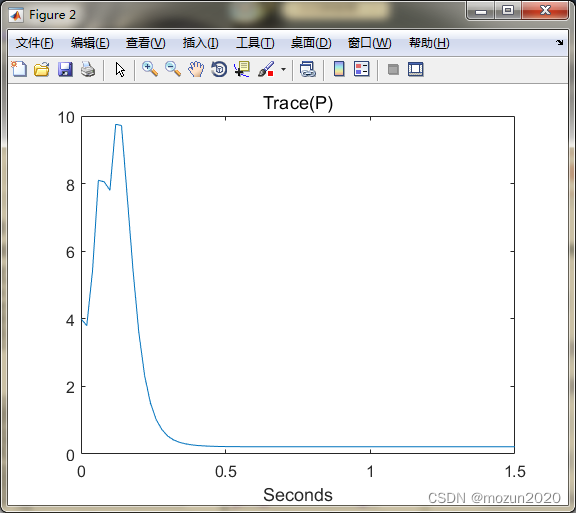
figure;
plot(tArray, trPArray); title('Trace(P)', 'FontSize', 12);
set(gca,'FontSize',12); set(gcf,'Color','White');
xlabel('Seconds');
% Compute the std dev of the estimation errors
N = size(xArray, 2);
N2 = round(N / 2);
xArray = xArray(:,N2:N);
xhatArray = xhatArray(:,N2:N);
iaEstErr = sqrt(norm(xArray(1,:)-xhatArray(1,:))^2 / size(xArray,2));
ibEstErr = sqrt(norm(xArray(2,:)-xhatArray(2,:))^2 / size(xArray,2));
wEstErr = sqrt(norm(xArray(3,:)-xhatArray(3,:))^2 / size(xArray,2));
thetaEstErr = sqrt(norm(xArray(4,:)-xhatArray(4,:))^2 / size(xArray,2));
disp(['Std Dev of Estimation Errors = ',num2str(iaEstErr),', ',num2str(ibEstErr),', ',num2str(wEstErr),', ',num2str(thetaEstErr)]);
% Display the P version of the estimation error standard deviations
disp(['Sqrt(P) = ',num2str(sqrt(P(1,1))),', ',num2str(sqrt(P(2,2))),', ',num2str(sqrt(P(3,3))),', ',num2str(sqrt(P(4,4)))]);

>> MotorKalman
Std Dev of Estimation Errors = 0.087107, 0.094443, 0.43097, 0.034275
Sqrt(P) = 0.093646, 0.093653, 0.44218, 0.025197
2. MATLAB仿真:示例13.2(1)
%%%%%%%%%%%%%%%%%%%%%%%%%%%%%%%%%%%%%%%%%%%%%%%%%%%%
%功能:《最优状态估计-卡尔曼,H∞及非线性滤波》示例仿真
%示例13.2: ExtendedBody.m
%环境:Win7,Matlab2015b
%Modi: C.S
%时间:2022-05-02
%%%%%%%%%%%%%%%%%%%%%%%%%%%%%%%%%%%%%%%%%%%%%%%%%%%%
function [AltErr, VelErr, BallErr] = ExtendedBody
% Continuous time etended Kalman filter example.
% Track a body falling through the atmosphere.
% Outputs are:
% AltErr = RMS altitude estimation error
% VelErr = RMS velocity estimation error
% BallErr = RMS ballistic coefficient estimation error
rho0 = 0.0034; % lb-sec^2/ft^4
g = 32.2; % ft/sec^2
k = 22000; % ft
R = 100; % measurement variance (ft^2)
x = [100000; -6000; 2000]; % initial state
xhat = [100010; -6100; 2500]; % initial state estimate
H = [1 0 0]; % measurement matrix
P = [500 0 0; 0 20000 0; 0 0 250000]; % initial estimation error covariance
tf = 16; % simulation length
dt = tf / 40000; % simulation step size
PlotStep = 200; % how often to plot data points
i = 0;
xArray = x;
xhatArray = xhat;
for t = dt : dt : tf
% Simulate the system (rectangular integration).
xdot(1,1) = x(2);
xdot(2,1) = rho0 * exp(-x(1)/k) * x(2)^2 / 2 / x(3) - g;
xdot(3,1) = 0;
x = x + xdot * dt;
% Simulate the measurement.
z = H * x + sqrt(R) * randn;
% Simulate the filter.
temp = rho0 * exp(-xhat(1)/k) * xhat(2) / xhat(3);
F = [0 1 0; -temp * xhat(2) / 2 / k temp ...
-temp * xhat(2) / 2 / xhat(3); ...
0 0 0];
Pdot = F * P + P * F' - P * H' * inv(R) * H * P;
P = P + Pdot * dt;
K = P * H' * inv(R);
xhatdot(1,1) = xhat(2);
xhatdot(2,1) = temp * xhat(2) / 2 - g;
xhatdot(3,1) = 0;
xhatdot = xhatdot + K * (z - H * xhat);
xhat = xhat + xhatdot * dt;
% Save data for plotting.
i = i + 1;
if i == PlotStep
xArray = [xArray x];
xhatArray = [xhatArray xhat];
i = 0;
end
end
% Plot data.
close all;
t = 0 : PlotStep*dt : tf;
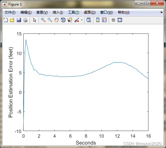
figure;
plot(t, xArray(1,:) - xhatArray(1,:));
set(gca,'FontSize',12); set(gcf,'Color','White');
xlabel('Seconds'); ylabel('Position Estimation Error (feet)');
AltErr = std(xArray(1,:) - xhatArray(1,:));
disp(['Continuous EKF RMS altitude estimation error = ', num2str(AltErr)]);
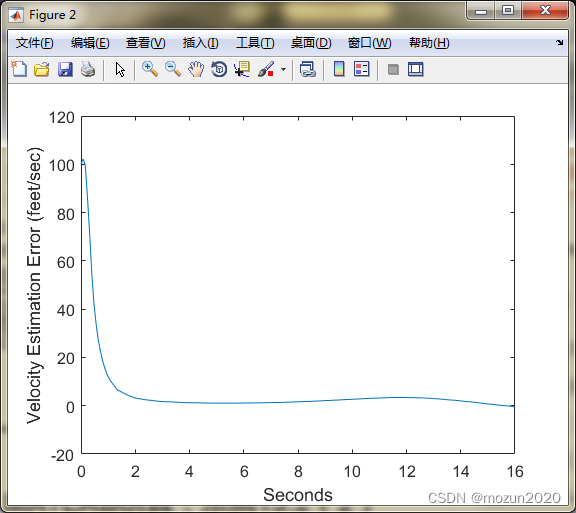
figure;
plot(t, xArray(2,:) - xhatArray(2,:));
set(gca,'FontSize',12); set(gcf,'Color','White');
xlabel('Seconds'); ylabel('Velocity Estimation Error (feet/sec)');
VelErr = std(xArray(2,:) - xhatArray(2,:));
disp(['Continuous EKF RMS velocity estimation error = ', num2str(VelErr)]);
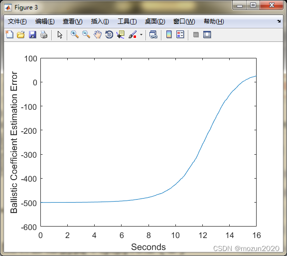
figure;
plot(t, xArray(3,:) - xhatArray(3,:));
set(gca,'FontSize',12); set(gcf,'Color','White');
xlabel('Seconds'); ylabel('Ballistic Coefficient Estimation Error');
BallErr = std(xArray(3,:) - xhatArray(3,:));
disp(['Continuous EKF RMS ballistic coefficient estimation error = ', num2str(BallErr)]);
figure;
plot(t, xArray(1,:));
title('Falling Body Simulation', 'FontSize', 12);
set(gca,'FontSize',12); set(gcf,'Color','White');
xlabel('Seconds'); ylabel('True Position');
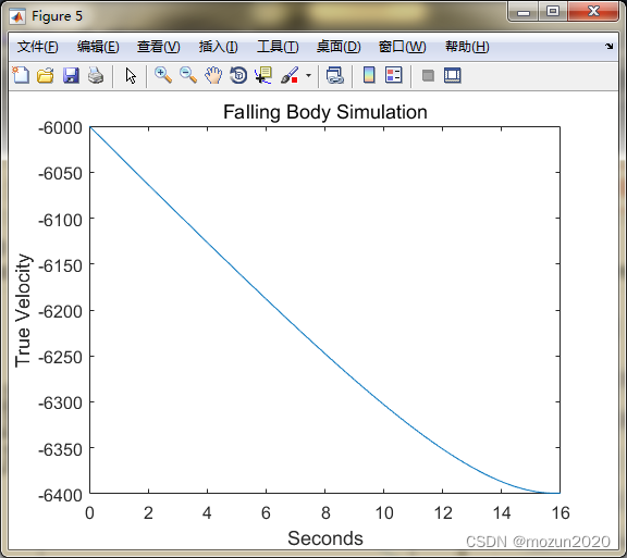
figure;
plot(t, xArray(2,:));
title('Falling Body Simulation', 'FontSize', 12);
set(gca,'FontSize',12); set(gcf,'Color','White');
xlabel('Seconds'); ylabel('True Velocity');

>> ExtendedBody
Continuous EKF RMS altitude estimation error = 2.1055
Continuous EKF RMS velocity estimation error = 15.1585
Continuous EKF RMS ballistic coefficient estimation error = 181.7602

ans =

    2.1055
3. MATLAB仿真:示例13.2(2)
%%%%%%%%%%%%%%%%%%%%%%%%%%%%%%%%%%%%%%%%%%%%%%%%%%%%
%功能:《最优状态估计-卡尔曼,H∞及非线性滤波》示例仿真
%示例13.2: HybridBody.m
%环境:Win7,Matlab2015b
%Modi: C.S
%时间:2022-05-02
%%%%%%%%%%%%%%%%%%%%%%%%%%%%%%%%%%%%%%%%%%%%%%%%%%%%
function [AltErr, VelErr, BallErr] = HybridBody
% Hybrid extended Kalman filter example.
% Track a body falling through the atmosphere.
% Outputs are:
% AltErr = RMS altitude estimation error
% VelErr = RMS velocity estimation error
% BallErr = RMS ballistic coefficient estimation error
rho0 = 0.0034; % lb-sec^2/ft^4
g = 32.2; % ft/sec^2
k = 22000; % ft
R = 100; % measurement variance (ft^2)
x = [100000; -6000; 2000]; % initial state
xhat = [100010; -6100; 2500]; % initial state estimate
H = [1 0 0]; % measurement matrix
P = [500 0 0; 0 20000 0; 0 0 250000];
T = 0.5; % measurement time step
tf = 16; % simulation length
dt = tf / 40000; % time step for integration
xArray = x;
xhatArray = xhat;
for t = T : T : tf
% Simulate the system.
for tau = dt : dt : T
xdot(1,1) = x(2);
xdot(2,1) = rho0 * exp(-x(1)/k) * x(2)^2 / 2 / x(3) - g;
xdot(3,1) = 0;
x = x + xdot * dt;
end
% Simulate the measurement.
z = H * x + sqrt(R) * randn;
% Simulate the continuous-time part of the filter.
for tau = dt : dt : T
xhatdot(1,1) = xhat(2);
xhatdot(2,1) = rho0 * exp(-xhat(1)/k) * xhat(2)^2 / 2 / xhat(3) - g;
xhatdot(3,1) = 0;
xhat = xhat + xhatdot * dt;
F = [0 1 0; -rho0 * exp(-xhat(1)/k) * xhat(2)^2 / 2 / k / xhat(3) ...
rho0 * exp(-xhat(1)/k) * xhat(2) / xhat(3) ...
-rho0 * exp(-xhat(1)/k) * xhat(2)^2 / 2 / xhat(3)^2; ...
0 0 0];
Pdot = F * P + P * F';
P = P + Pdot * dt;
end
% Simulate the discrete-time part of the filter.
K = P * H' * inv(H * P * H' + R);
xhat = xhat + K * (z - H * xhat);
P = (eye(3) - K * H) * P * (eye(3) - K * H)' + K * R * K';
% Save data for plotting.
xArray = [xArray x];
xhatArray = [xhatArray xhat];
end
% Plot data
close all;
t = 0 : T : tf;
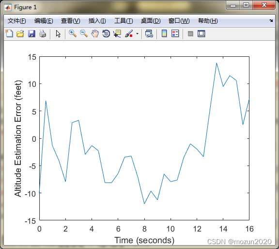
figure;
plot(t, xArray(1,:) - xhatArray(1,:));
set(gca,'FontSize',12); set(gcf,'Color','White');
xlabel('Time (seconds)');
ylabel('Altitude Estimation Error (feet)');
AltErr = std(xArray(1,:) - xhatArray(1,:));
disp(['Hybrid EKF RMS altitude estimation error = ', num2str(AltErr)]);
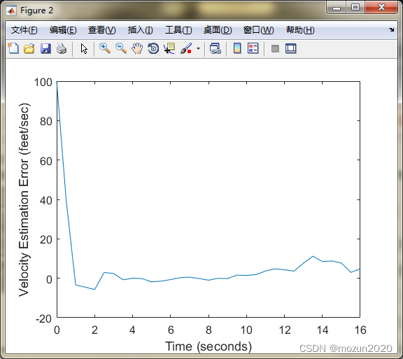
figure;
plot(t, xArray(2,:) - xhatArray(2,:));
set(gca,'FontSize',12); set(gcf,'Color','White');
xlabel('Time (seconds)');
ylabel('Velocity Estimation Error (feet/sec)');
VelErr = std(xArray(2,:) - xhatArray(2,:));
disp(['Hybrid EKF RMS velocity estimation error = ', num2str(VelErr)]);
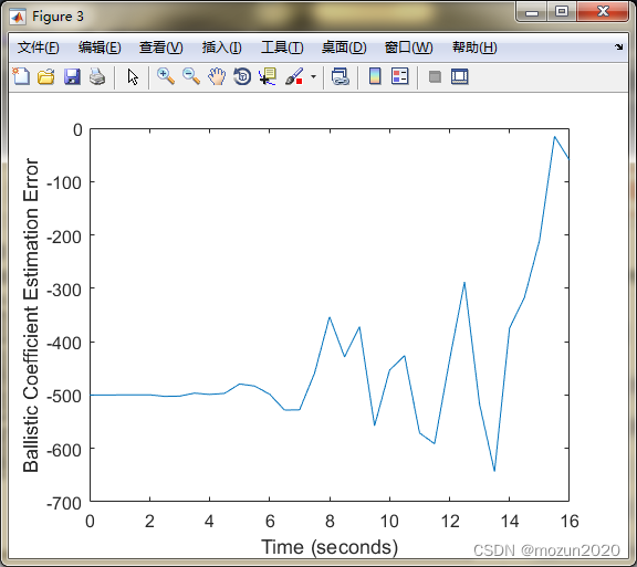
figure;
plot(t, xArray(3,:) - xhatArray(3,:));
set(gca,'FontSize',12); set(gcf,'Color','White');
xlabel('Time (seconds)');
ylabel('Ballistic Coefficient Estimation Error');
BallErr = std(xArray(3,:) - xhatArray(3,:));
disp(['Hybrid EKF RMS ballistic coefficient estimation error = ', num2str(BallErr)]);
figure;
plot(t, xArray(1,:)/1000);
set(gca,'FontSize',12); set(gcf,'Color','White');
xlabel('Time (seconds)');
ylabel('True Altitude (thousands of feet)');
figure;
plot(t, xArray(2,:));
set(gca,'FontSize',12); set(gcf,'Color','White');
xlabel('Time (seconds)');
ylabel('True Velocity (feet/sec)');


>> HybridBody
Hybrid EKF RMS altitude estimation error = 7.02
Hybrid EKF RMS velocity estimation error = 18.5111
Hybrid EKF RMS ballistic coefficient estimation error = 136.0415

ans =

    7.0200
4. MATLAB仿真:示例13.3
%%%%%%%%%%%%%%%%%%%%%%%%%%%%%%%%%%%%%%%%%%%%%%%%%%%%
%功能:《最优状态估计-卡尔曼,H∞及非线性滤波》示例仿真
%示例13.3: Hybrid2.m
%环境:Win7,Matlab2015b
%Modi: C.S
%时间:2022-05-02
%%%%%%%%%%%%%%%%%%%%%%%%%%%%%%%%%%%%%%%%%%%%%%%%%%%%
function [EKFErr, EKF2Err, EKFiErr] = Hybrid2
% Optimal State Estimation, by Dan Simon
%
% Hybrid second order Kalman filter example.
% Track a body falling through the atmosphere.
% This example is taken from [Ath68].
% Outputs:
% EKFErr = 1st order EKF estimation error (RMS) (altitude, velocity, ballistic coefficient)
% EKF2Err = 2nd order EKF estimation error (RMS) (altitude, velocity, ballistic coefficient)
% EKFiErr = iterated EKF estimation error (RMS) (altitude, velocity, ballistic coefficient)
% Revision March 3, 2009 - The Q terms were being incorrectly multiplied by dt in the RungeKutta routine,
% which was incorrect (although it does not affect the results in this case since Q = 0).
global rho0 g k dt
rho0 = 2; % lb-sec^2/ft^4
g = 32.2; % ft/sec^2
k = 2e4; % ft
R = 10^4; % measurement noise variance (ft^2)
Q = diag([0 0 0]); % process noise covariance
M = 10^5; % horizontal range of position sensor
a = 10^5; % altitude of position sensor
x = [3e5; -2e4; 1e-3]; % true state
xhat = [3e5; -2e4; 1e-3]; % first order EKF estimate
xhat2 = xhat; % second order EKF estimate
xhati = xhat; % iterated EKF estimate
N = 7; % max number of iterations to execute in the iterated EKF
P = diag([1e6 4e6 10]);
P2 = P;
Pi = P;
T = 1; % measurement time step
randn('state',sum(100*clock)); % random number generator seed
tf = 30; % simulation length (seconds)
dt = 0.02; % time step for integration (seconds)
xArray = x;
xhatArray = xhat;
xhat2Array = xhat2;
xhatiArray = xhati;
Parray = diag(P);
P2array = diag(P2);
Piarray = diag(Pi);
for t = T : T : tf
% Simulate the system.
for tau = dt : dt : T
% Fourth order Runge Kutta ingegration
[dx1, dx2, dx3, dx4] = RungeKutta(x);
x = x + (dx1 + 2 * dx2 + 2 * dx3 + dx4) / 6;
x = x + sqrt(dt * Q) * [randn; randn; randn] * dt;
end
% Simulate the noisy measurement.
z = sqrt(M^2 + (x(1)-a)^2) + sqrt(R) * randn;
% First order Kalman filter.
% Simulate the continuous-time part of the first order Kalman filter (time update).
for tau = dt : dt : T
[dx1, dx2, dx3, dx4] = RungeKutta(xhat);
xhat = xhat + (dx1 + 2 * dx2 + 2 * dx3 + dx4) / 6;
F = [0 1 0; -rho0 * exp(-xhat(1)/k) * xhat(2)^2 / 2 / k * xhat(3) ...
rho0 * exp(-xhat(1)/k) * xhat(2) * xhat(3) ...
rho0 * exp(-xhat(1)/k) * xhat(2)^2 / 2; ...
0 0 0];
H = [(xhat(1) - a) / sqrt(M^2 + (xhat(1)-a)^2) 0 0];
[dP1, dP2, dP3, dP4] = RungeKuttaP(P, F, Q, dt, H, R);
P = P + (dP1 + 2 * dP2 + 2 * dP3 + dP4) / 6;
end
% Force the ballistic coefficient estimate to be non-negative.
xhat(3) = max(xhat(3), 0);
% Simulate the discrete-time part of the first order Kalman filter (measurement update).
H = [(xhat(1) - a) / sqrt(M^2 + (xhat(1)-a)^2) 0 0];
K = P * H' * inv(H * P * H' + R);
zhat = sqrt(M^2 + (xhat(1)-a)^2);
xhat = xhat + K * (z - zhat);
% Force the ballistic coefficient estimate to be non-negative.
xhat(3) = max(xhat(3), 0);
P = (eye(3) - K * H) * P;
% Iterated Kalman filter.
% Simulate the continuous-time part of the iterated Kalman filter (time update).
for tau = dt : dt : T
[dx1, dx2, dx3, dx4] = RungeKutta(xhati);
xhati = xhati + (dx1 + 2 * dx2 + 2 * dx3 + dx4) / 6;
F = [0 1 0; -rho0 * exp(-xhati(1)/k) * xhati(2)^2 / 2 / k * xhati(3) ...
rho0 * exp(-xhati(1)/k) * xhati(2) * xhati(3) ...
rho0 * exp(-xhati(1)/k) * xhati(2)^2 / 2; ...
0 0 0];
H = [(xhati(1) - a) / sqrt(M^2 + (xhati(1)-a)^2) 0 0];
[dP1, dP2, dP3, dP4] = RungeKuttaP(Pi, F, Q, dt, H, R);
Pi = Pi + (dP1 + 2 * dP2 + 2 * dP3 + dP4) / 6;
end
% Force the ballistic coefficient estimate to be non-negative.
xhati(3) = max(xhati(3), 0);
% Simulate the discrete time part of the iterated Kalman filter (measurement update);
xhatminus = xhati;
Pminus = Pi;
for i = 1 : N
H = [(xhati(1) - a) / sqrt(M^2 + (xhati(1)-a)^2) 0 0];
K = Pminus * H' * inv(H * Pminus * H' + R);
zhat = sqrt(M^2 + (xhati(1)-a)^2);
xhati = xhatminus + K * ((z - zhat) - H * (xhatminus - xhati));
Pi = (eye(3) - K * H) * Pminus;
% Force the ballistic coefficient estimate to be non-negative.
xhati(3) = max(xhati(3), 0);
end
% Second order Kalman filter.
% Simulate the continuous-time part of the second order Kalman filter (time update).
for tau = dt : dt : T
[dx, dP] = RungeKutta2(xhat2, P2, Q, R);
xhat2 = xhat2 + (dx(:,1) + 2 * dx(:,2) + 2 * dx(:,3) + dx(:,4)) / 6;
P2 = P2 + (dP(:,:,1) + 2 * dP(:,:,2) + 2 * dP(:,:,3) + dP(:,:,4)) / 6;
end
% Force the ballistic coefficient estimate to be non-negative.
xhat2(3) = max(xhat2(3), 0);
% Simulate the discrete-time part of the second order Kalman filter (measurement update).
H = [(xhat2(1) - a) / sqrt(M^2 + (xhat2(1)-a)^2) 0 0];
zhat = sqrt(M^2 + (xhat2(1)-a)^2);
D = zeros(3,3);
D(1,1) = 1/zhat * (1 - (xhat2(1) - a)^2 / zhat / zhat);
L = 1/2 * trace(D * P2 * D * P2);
K = P2 * H' * inv(H * P2 * H' + R + L);
pie = 1/2 * K * [1] * trace(D * P2);
xhat2 = xhat2 + K * (z - zhat) - pie;
% Force the ballistic coefficient estimate to be non-negative.
xhat2(3) = max(xhat2(3), 0);
P2 = P2 - P2 * H' * (H * P2 * H' + R + L)^(-1) * H * P2;
% Save data for plotting.
xArray = [xArray x];
xhatArray = [xhatArray xhat];
xhat2Array = [xhat2Array xhat2];
xhatiArray = [xhatiArray xhati];
Parray = [Parray diag(P)];
P2array = [P2array diag(P2)];
Piarray = [Piarray diag(Pi)];
end
close all;
t = 0 : T : tf;
figure;
semilogy(t, abs(xArray(1,:) - xhatArray(1,:)), 'b', 'LineWidth', 2); hold;
semilogy(t, abs(xArray(1,:) - xhat2Array(1,:)), 'r:', 'LineWidth', 2);
semilogy(t, abs(xArray(1,:) - xhatiArray(1,:)), 'k--', 'LineWidth', 2);
set(gca,'FontSize',12); set(gcf,'Color','White');
xlabel('Seconds');
ylabel('Altitude Estimation Error');
legend('Kalman filter', 'Second order filter', 'Iterated Kalman filter');
AltErr = std(xArray(1,:) - xhatArray(1,:));
disp(['1st Order EKF RMS altitude estimation error = ', num2str(AltErr)]);
Alt2Err = std(xArray(1,:) - xhat2Array(1,:));
disp(['2nd Order EKF RMS altitude estimation error = ', num2str(Alt2Err)]);
AltiErr = std(xArray(1,:) - xhatiArray(1,:));
disp(['Iterated EKF RMS altitude estimation error = ', num2str(AltiErr)]);
figure;
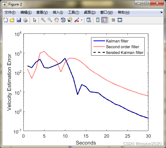
semilogy(t, abs(xArray(2,:) - xhatArray(2,:)), 'b', 'LineWidth', 2); hold;
semilogy(t, abs(xArray(2,:) - xhat2Array(2,:)), 'r:', 'LineWidth', 2);
semilogy(t, abs(xArray(2,:) - xhatiArray(2,:)), 'k--', 'LineWidth', 2);
set(gca,'FontSize',12); set(gcf,'Color','White');
xlabel('Seconds');
ylabel('Velocity Estimation Error');
legend('Kalman filter', 'Second order filter', 'Iterated Kalman filter');
VelErr = std(xArray(2,:) - xhatArray(2,:));
disp(['1st Order EKF RMS velocity estimation error = ', num2str(VelErr)]);
Vel2Err = std(xArray(2,:) - xhat2Array(2,:));
disp(['2nd Order EKF RMS velocity estimation error = ', num2str(Vel2Err)]);
VeliErr = std(xArray(2,:) - xhatiArray(2,:));
disp(['Iterated EKF RMS velocity estimation error = ', num2str(VeliErr)]);
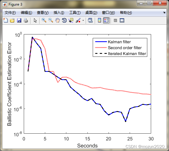
figure;
semilogy(t, abs(xArray(3,:) - xhatArray(3,:)), 'b', 'LineWidth', 2); hold;
semilogy(t, abs(xArray(3,:) - xhat2Array(3,:)), 'r:', 'LineWidth', 2);
semilogy(t, abs(xArray(3,:) - xhatiArray(3,:)), 'k--', 'LineWidth', 2);
set(gca,'FontSize',12); set(gcf,'Color','White');
xlabel('Seconds');
ylabel('Ballistic Coefficient Estimation Error');
legend('Kalman filter', 'Second order filter', 'Iterated Kalman filter');
BallErr = std(xArray(3,:) - xhatArray(3,:));
disp(['1st Order EKF RMS ballistic coefficient estimation error = ', num2str(BallErr)]);
Ball2Err = std(xArray(3,:) - xhat2Array(3,:));
disp(['2nd Order EKF RMS ballistic coefficient estimation error = ', num2str(Ball2Err)]);
BalliErr = std(xArray(3,:) - xhatiArray(3,:));
disp(['Iterated EKF RMS ballistic coefficient estimation error = ', num2str(BalliErr)]);
figure;
plot(t, xArray(1,:), 'LineWidth', 2);
set(gca,'FontSize',12); set(gcf,'Color','White');
xlabel('Seconds');
ylabel('True Altitude');
grid;
figure;
plot(t, xArray(2,:), 'LineWidth', 2);
title('Falling Body Simulation', 'FontSize', 12);
set(gca,'FontSize',12); set(gcf,'Color','White');
xlabel('Seconds');
ylabel('True Velocity');
grid;
EKFErr = [AltErr; VelErr; BallErr];
EKF2Err = [Alt2Err; Vel2Err; Ball2Err];
EKFiErr = [AltiErr; VeliErr; BalliErr];
return
%%%%%%%%%%%%%%%%%%%%%%%%%%%%%%%%%%%%%%%%%%%%%%
function [dx1, dx2, dx3, dx4] = RungeKutta(x)
% Fourth order Runge Kutta integration for the falling body system.
global rho0 g k dt
dx1(1,1) = x(2);
dx1(2,1) = rho0 * exp(-x(1)/k) * x(2)^2 / 2 * x(3) - g;
dx1(3,1) = 0;
dx1 = dx1 * dt;
xtemp = x + dx1 / 2;
dx2(1,1) = xtemp(2);
dx2(2,1) = rho0 * exp(-xtemp(1)/k) * xtemp(2)^2 / 2 * xtemp(3) - g;
dx2(3,1) = 0;
dx2 = dx2 * dt;
xtemp = x + dx2 / 2;
dx3(1,1) = xtemp(2);
dx3(2,1) = rho0 * exp(-xtemp(1)/k) * xtemp(2)^2 / 2 * xtemp(3) - g;
dx3(3,1) = 0;
dx3 = dx3 * dt;
xtemp = x + dx3;
dx4(1,1) = xtemp(2);
dx4(2,1) = rho0 * exp(-xtemp(1)/k) * xtemp(2)^2 / 2 * xtemp(3) - g;
dx4(3,1) = 0;
dx4 = dx4 * dt;
return
%%%%%%%%%%%%%%%%%%%%%%%%%%%%%%%%%%%%%%%%%%%%%%%%%%%
function [dx, dP] = RungeKutta2(x, P, Q, R)
% Fourth order Runge Kutta integration for the falling body system for the second order Kalman filter estimate.
global rho0 g k dt
% First Runge Kutta increment for x and P.
xtemp = x;
Ptemp = P;
exp1 = exp(-xtemp(1) / k);
F = [0 1 0; -rho0 * exp1 * xtemp(2)^2 / 2 / k * xtemp(3) ...
rho0 * exp1 * xtemp(2) * xtemp(3) ...
rho0 * exp1 * xtemp(2)^2 / 2; ...
0 0 0];
F1 = zeros(3,3);
F2 = [rho0 / k / k * exp1 * xtemp(2)^2 / 2 * xtemp(3) -rho0 / k * exp1 * xtemp(2) * xtemp(3) -rho0 / k * exp1 * xtemp(2)^2 / 2 ;
-rho0 / k * exp1 * xtemp(2) * x(3) rho0 * exp1 * xtemp(3) rho0 * exp(-xtemp(1) / k) * xtemp(2) ;
-rho0 / k * exp1 * xtemp(2)^2 / 2 rho0 * exp1 * xtemp(2) 0 ];
F3 = zeros(3,3);
ubreve = 1/2 * ([1 ; 0 ; 0] * trace(F1 * Ptemp) + [0 ; 1 ; 0] * trace(F2 * Ptemp) + [0 ; 0 ; 1] * trace(F3 * Ptemp));
dx(1,1) = xtemp(2);
dx(2,1) = rho0 * exp(-xtemp(1)/k) * xtemp(2)^2 / 2 * xtemp(3) - g;
dx(3,1) = 0;
dx(:,1) = (dx(:,1) + ubreve) * dt;
xtemp = x + dx(:,1) / 2;
dP(:,:,1) = F * Ptemp + Ptemp * F' + Q * dt;
dP(:,:,1) = dP(:,:,1) * dt;
Ptemp = P + dP(:,:,1) / 2;
% Second Runge Kutta increment for x and P.
exp1 = exp(-xtemp(1) / k);
F = [0 1 0; -rho0 * exp1 * xtemp(2)^2 / 2 / k * xtemp(3) ...
rho0 * exp1 * xtemp(2) * xtemp(3) ...
rho0 * exp1 * xtemp(2)^2 / 2; ...
0 0 0];
F1 = zeros(3,3);
F2 = [rho0 / k / k * exp1 * xtemp(2)^2 / 2 * xtemp(3) -rho0 / k * exp1 * xtemp(2) * xtemp(3) -rho0 / k * exp1 * xtemp(2)^2 / 2 ;
-rho0 / k * exp1 * xtemp(2) * x(3) rho0 * exp1 * xtemp(3) rho0 * exp(-xtemp(1) / k) * xtemp(2) ;
-rho0 / k * exp1 * xtemp(2)^2 / 2 rho0 * exp1 * xtemp(2) 0 ];
F3 = zeros(3,3);
ubreve = 1/2 * ([1 ; 0 ; 0] * trace(F1 * Ptemp) + [0 ; 1 ; 0] * trace(F2 * Ptemp) + [0 ; 0 ; 1] * trace(F3 * Ptemp));
dx(1,2) = xtemp(2);
dx(2,2) = rho0 * exp(-xtemp(1)/k) * xtemp(2)^2 / 2 * xtemp(3) - g;
dx(3,2) = 0;
dx(:,2) = (dx(:,2) + ubreve) * dt;
xtemp = x + dx(:,2) / 2;
dP(:,:,2) = F * Ptemp + Ptemp * F' + Q * dt;
dP(:,:,2) = dP(:,:,2) * dt;
Ptemp = P + dP(:,:,2) / 2;
% Third Runge Kutta increment for x and P.
exp1 = exp(-xtemp(1) / k);
F = [0 1 0; -rho0 * exp1 * xtemp(2)^2 / 2 / k * xtemp(3) ...
rho0 * exp1 * xtemp(2) * xtemp(3) ...
rho0 * exp1 * xtemp(2)^2 / 2; ...
0 0 0];
F1 = zeros(3,3);
F2 = [rho0 / k / k * exp1 * xtemp(2)^2 / 2 * xtemp(3) -rho0 / k * exp1 * xtemp(2) * xtemp(3) -rho0 / k * exp1 * xtemp(2)^2 / 2 ;
-rho0 / k * exp1 * xtemp(2) * x(3) rho0 * exp1 * xtemp(3) rho0 * exp(-xtemp(1) / k) * xtemp(2) ;
-rho0 / k * exp1 * xtemp(2)^2 / 2 rho0 * exp1 * xtemp(2) 0 ];
F3 = zeros(3,3);
ubreve = 1/2 * ([1 ; 0 ; 0] * trace(F1 * Ptemp) + [0 ; 1 ; 0] * trace(F2 * Ptemp) + [0 ; 0 ; 1] * trace(F3 * Ptemp));
dx(1,3) = xtemp(2);
dx(2,3) = rho0 * exp(-xtemp(1)/k) * xtemp(2)^2 / 2 * xtemp(3) - g;
dx(3,3) = 0;
dx(:,3) = (dx(:,3) + ubreve) * dt;
xtemp = x + dx(:,3);
dP(:,:,3) = F * Ptemp + Ptemp * F' + Q * dt;
dP(:,:,3) = dP(:,:,3) * dt;
Ptemp = P + dP(:,:,3);
% Fourth Runge Kutta increment for x and P.
exp1 = exp(-xtemp(1) / k);
F = [0 1 0; -rho0 * exp1 * xtemp(2)^2 / 2 / k * xtemp(3) ...
rho0 * exp1 * xtemp(2) * xtemp(3) ...
rho0 * exp1 * xtemp(2)^2 / 2; ...
0 0 0];
F1 = zeros(3,3);
F2 = [rho0 / k / k * exp1 * xtemp(2)^2 / 2 * xtemp(3) -rho0 / k * exp1 * xtemp(2) * xtemp(3) -rho0 / k * exp1 * xtemp(2)^2 / 2 ;
-rho0 / k * exp1 * xtemp(2) * x(3) rho0 * exp1 * xtemp(3) rho0 * exp(-xtemp(1) / k) * xtemp(2) ;
-rho0 / k * exp1 * xtemp(2)^2 / 2 rho0 * exp1 * xtemp(2) 0 ];
F3 = zeros(3,3);
ubreve = 1/2 * ([1 ; 0 ; 0] * trace(F1 * Ptemp) + [0 ; 1 ; 0] * trace(F2 * Ptemp) + [0 ; 0 ; 1] * trace(F3 * Ptemp));
dx(1,4) = xtemp(2);
dx(2,4) = rho0 * exp(-xtemp(1)/k) * xtemp(2)^2 / 2 * xtemp(3) - g;
dx(3,4) = 0;
dx(:,4) = (dx(:,4) + ubreve) * dt;
dP(:,:,4) = F * Ptemp + Ptemp * F' + Q * dt;
dP(:,:,4) = dP(:,:,4) * dt;
return
%%%%%%%%%%%%%%%%%%%%%%%%%%%%%%%%%%%%%%%%%%%%%%%%%%%%%%%%%%%%%%%%%%%
function [dP1, dP2, dP3, dP4] = RungeKuttaP(P, F, Q, dt, H, R)
% Fourth order Runge Kutta integration for the covariance of the Kalman
% filter for the falling body system.
dP1 = F * P + P * F' + Q - P * H' * inv(R) * H * P;
dP1 = dP1 * dt;
Ptemp = P + dP1 / 2;
dP2 = F * Ptemp + Ptemp * F' + Q - Ptemp * H' * inv(R) * H * Ptemp;
dP2 = dP2 * dt;
Ptemp = P + dP2 / 2;
dP3 = F * Ptemp + Ptemp * F' + Q - Ptemp * H' * inv(R) * H * Ptemp;
dP3 = dP3 * dt;
Ptemp = P + dP3;
dP4 = F * Ptemp + Ptemp * F' + Q - Ptemp * H' * inv(R) * H * Ptemp;
dP4 = dP4 * dt;
return


>> Hybrid2
已锁定最新绘图
1st Order EKF RMS altitude estimation error = 214.6258
2nd Order EKF RMS altitude estimation error = 171.5054
Iterated EKF RMS altitude estimation error = 213.8927
已锁定最新绘图
1st Order EKF RMS velocity estimation error = 182.5166
2nd Order EKF RMS velocity estimation error = 356.8217
Iterated EKF RMS velocity estimation error = 182.4223
已锁定最新绘图
1st Order EKF RMS ballistic coefficient estimation error = 0.11202
2nd Order EKF RMS ballistic coefficient estimation error = 0.11767
Iterated EKF RMS ballistic coefficient estimation error = 0.11202

ans =

  214.6258
  182.5166
    0.1120
4. MATLAB仿真:示例13.4
%%%%%%%%%%%%%%%%%%%%%%%%%%%%%%%%%%%%%%%%%%%%%%%%%%%%
%功能:《最优状态估计-卡尔曼,H∞及非线性滤波》示例仿真
%示例13.4: Parameter.m
%环境:Win7,Matlab2015b
%Modi: C.S
%时间:2022-05-02
%%%%%%%%%%%%%%%%%%%%%%%%%%%%%%%%%%%%%%%%%%%%%%%%%%%%

function Parameter

% Extended Kalman filter for parameter estimation.
% Estimate the natural frequency of a second order system.

tf = 100; % simulation length
dt = 0.01; % simulation step size
wn = 2; % natural frequency
zeta = 0.1; % damping ratio
b = -2 * zeta * wn;
Q2 = 0.1; % artificial noise used for parameter estimation
Q2 = 1;

Q = [1000 0; 0 Q2]; % covariance of process noise
R = [10 0; 0 10]; % covariance of measurement noise
H = [1 0 0; 0 1 0]; % measurement matrix
P = [0 0 0; 0 0 0; 0 0 20]; % covariance of estimation error

x = [0; 0; -wn*wn]; % initial state
xhat = 2 * x; % initial state estimate

% Initialize arrays for later plotting
xArray = x;
xhatArray = xhat;
P3Array = P(3,3);

dtPlot = tf / 100; % how often to plot output data
tPlot = 0;

for t = dt : dt : tf+dt
    % Simulate the system.
    w = sqrt(Q(1,1)) * randn;
    xdot = [x(2); x(3)*x(1) + b*x(2) - x(3)*w; 0];
    x = x + xdot * dt;
    z = H * x + sqrt(R) * [randn; randn];
    % Simulate the Kalman filter.
    F = [0 1 0; xhat(3) b xhat(1); 0 0 0];
    L = [0 0; -xhat(3) 0; 0 1];
    Pdot = F * P + P * F' + L * Q * L' - P * H' * inv(R) * H * P;
    P = P + Pdot * dt;
    K = P * H' * inv(R);
    xhatdot = [xhat(2); xhat(3)*xhat(1) + b*xhat(2); 0];
    xhatdot = xhatdot + K * (z - H * xhat);
    xhat = xhat + xhatdot * dt;
    if (t >= tPlot + dtPlot - 100*eps)
        % Save data for plotting.
        xArray = [xArray x];
        xhatArray = [xhatArray xhat];
        P3Array = [P3Array P(3,3)];
        tPlot = t;
    end
end

% Plot results
close all
t = 0 : dtPlot : tf;

figure;
plot(t, xArray(3,:) - xhatArray(3,:));
set(gca,'FontSize',12); set(gcf,'Color','White');
xlabel('Seconds'); ylabel('w_n^2 Estimation Error');

figure;
plot(t, P3Array);
set(gca,'FontSize',12); set(gcf,'Color','White');
xlabel('Seconds'); ylabel('Variance of w_n^2 Estimation Error');

disp(['Final estimation error = ', num2str(xArray(3,end)-xhatArray(3,end))]);
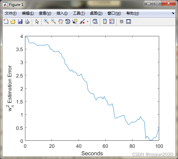

>> Parameter
Final estimation error = 0.49938
5. 小结
运动控制在现代生活中的实际应用非常广泛,除了智能工厂中各种智能设备的自动运转控制,近几年最火的自动驾驶技术,以及航空航天领域,都缺少不了它的身影,所以熟练掌握状态估计理论,对未来就业也是非常有帮助的。切记矩阵理论与概率论等知识的基础一定要打好。对本章内容感兴趣或者想充分学习了解的,建议去研习书中第十三章节的内容,有条件的可以通过习题的联系进一步巩固充实。后期会对其中一些知识点在自己理解的基础上进行讨论补充,欢迎大家一起学习交流。
原书链接:Optimal State Estimation:Kalman, H-infinity, and Nonlinear Approaches
本文内容由网友自发贡献,版权归原作者所有,本站不承担相应法律责任。如您发现有涉嫌抄袭侵权的内容,请联系:hwhale#tublm.com(使用前将#替换为@)